In Chapter 1 and Chapter 2, you have encountered applications related to velocity and distance, pollution, temperature, population growth, and natural resources. In this chapter, I present some applications in economics and finance, probability and statistics, along with numerical integration.
Although you gain access to some of these applications, these applications depend on simplifying assumptions which may or may not be stated explicitly. We may not have the time to actually go through the plausibility of these assumptions and they will be the responsibility of other instructors of courses which rely on these applications.
Most of the presented applications have also been stripped to their core components in order for you to be able to apply what you have learned so far.
4.1 Economics and finance
4.1.1 Bank accounts
At this stage, you know enough about how to set up differential equations and how to evaluate integrals. You can now apply these skills in some finance applications.
Activity
Congratulations, you just won the lottery! In one option presented to you, you will be paid one million dollars a year for the next 25 years. You can deposit this money in an account that will earn 5% each year.
Set up a differential equation that describes the rate of change in the amount of money in the account. Two factors cause the amount to grow—first, you are depositing one millon dollars per year and second, you are earning 5% interest.
If there is no amount of money in the account when you open it, how much money will you have in the account after 25 years?
The second option presented to you is to take a lump sum of 10 million dollars, which you will deposit into a similar account. How much money will you have in that account after 25 years?
Do you prefer the first or second option? Explain your thinking.
At what time does the amount of money in the account under the first option overtake the amount of money in the account under the second option?
4.1.2 Effect of an import ban on welfare
A classic application of integration is when we want to calculate the effect of market distortions on welfare. Consider a market for a good which a country imports and also produces domestically. An import ban is suddenly imposed on this market. How can we calculate the impact on welfare?
The idea is to compare welfare without the import ban against welfare with the import ban. For the comparison, we impose the following conditions:
The importing country is a price taker.
Transportation costs are equal to zero.
The effect of the import ban on other countries is ignored.
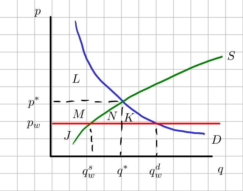
The resulting supply-demand diagrams are illustrated in Figure 4.1 and Figure 4.2. Let \(p_w\) be the price of the good outside of the domestic market. This will be the import price. The quantity supplied domestically is given by \(q_w^s\) and the quantity demanded domestically is given by \(q_w^d\). The total quantity imported is \(q_w^d-q_w^s\).
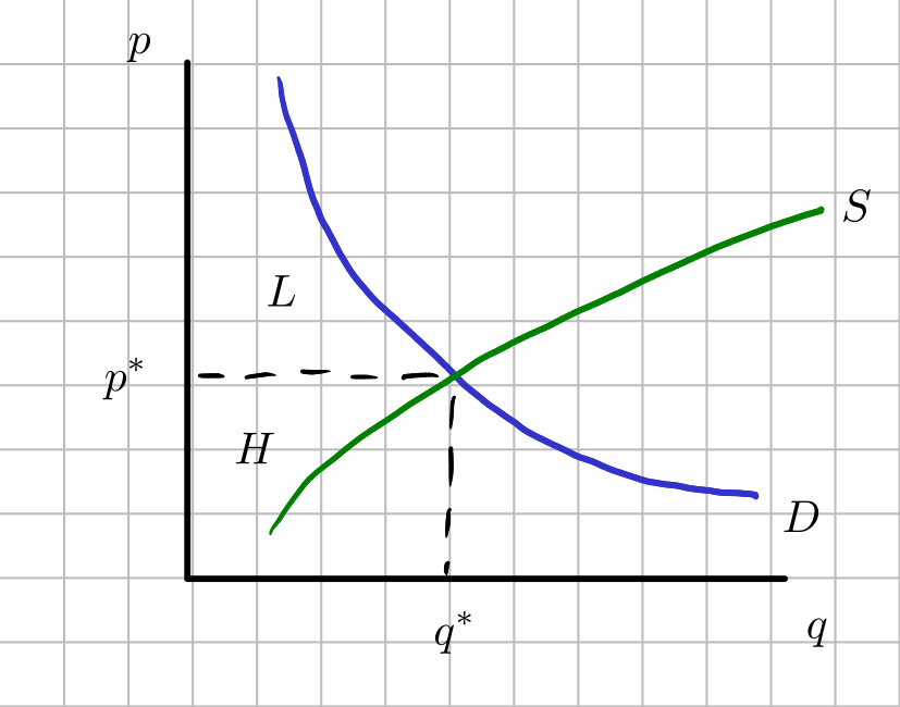
An import ban means that we could no longer import the good at \(p_w\). Let \(p^*\) and \(q^*\) be the domestic equilibrium price with the import ban. Clearly, \(p_w\) has to be less than \(p^*\) for importing to take place and for imposing an import ban to make sense (Why?). The import ban leads to domestic prices rising to \(p^*\) and domestic quantities reduced to \(q^*\).
Figure 4.1: Market conditions without import ban
Figure 4.2: Market conditions with import ban
The table below summarizes the consumer surplus and producer surplus with and without the import ban. The letters \(H\), \(J\), \(K\), \(L\), \(M\), and \(N\) are areas. Total welfare is equal to the sum of consumer surplus and producer surplus. The column Difference shows who gains and loses from the import ban. The entry \(-(N+K)\) in the table can be interpreted as a loss of welfare. This loss of welfare is called a deadweight loss because the gains by producers are not enough to offset the losses shouldered by consumers. Under our setting, it does not make sense to impose an import ban on goods, even if the good is being produced domestically.
Without import ban
With import ban
Difference
Consumer surplus
\(L+M+N+K\)
\(L\)
\(-(M+N+K)\)
Producer surplus
\(J\)
\(H=M+J\)
\(M\)
Welfare
\(L+M+N+K+J\)
\(L+M+J\)
\(-(N+K)\)
So far, the analysis shown is at the level of a principles course in economics. If you had to actually calculate consumer surplus, producer surplus, or deadweight losses, then you need a way to calculate the relevant areas.
To calculate (or at least to setup the expressions for) the relevant areas, we have to apply integration to write down the relevant expressions for the areas. We also use the ideas found in Exercise 7 of Section 2.3.3.
Let \(D(p)\) be the demand function and \(S(p)\) be the supply function. These expressions may feel strange in light of the plots found in Figure 4.1 and Figure 4.2. Observe that if you directly apply what we have learned and to match with the plots, we really should compute the inverse demand and inverse supply functions in order to express prices as functions of quantities. Unfortunately, the typical approach in economics is to work with \(D(p)\) and \(S(p)\), namely quantities as functions of prices. To adjust for this, you would have to consider the horizontal rectangular strips instead of vertical strips like we used to do before in Section 2.2 if you are going to use Riemann sums.
Once you are comfortable with this re-orientation, then you can obtain the following using what you have learned so far in Chapter 2: \[\begin{eqnarray*}M+N+K &=& \int_{p_w}^{p^*} D(p)\,dp \\ M&=& \int_{p_w}^{p^*} S(p)\,dp \\
\Rightarrow N+K &=& \int_{p_w}^{p^*} \left(D(p)-S(p)\right)\,dp\end{eqnarray*}\]
Although the definite integral used to calculate \(N+K\) is the correct area, the economic aspect of our setting requires us to take the negative of this area. Therefore, the resulting deadweight loss of the import ban is \[-(N+K)=-\int_{p_w}^{p^*} \left(D(p)-S(p)\right)\,dp.\]
There is not much we can do about \(-(N+K)\) unless we have some values of \(p_w\), \(p^*\) and the functional forms of \(D(p)\) and \(S(p)\). Where would you obtain them? The cheapest way is to just provide fictional numerical values and functional forms. Another way is to provide some basis for these values using data from real-life situations. You will be studying a course called econometrics and in that course, you may learn some techniques to allow you to estimate \(D(p)\) and \(S(p)\) using real data. Once you have these estimates and after some further work, you will be able to at least get a numerical value for \(-(N+K)\) for a particular context.
4.1.3 Solow growth model
When you reach the point where you study intermediate macroeconomics, you will be studying what makes countries grow and whether poor countries would eventually catch up to rich countries. One particular economic model used in the previously described setting is the Solow growth model.
4.1.3.1 Setup
For our purposes, we will only focus on the differential equation which is the core of the Solow growth model. We have to introduce the following elements:
\(k>0\) is the level of aggregate physical capital stock per capita.
\(y=f\left(k\right)\) is the aggregate production function1 in terms of aggregate capital stock per capita. \(y\) also represents the aggregate output per capita. We assume that \(f(0)=0\) with \(f(k)>0\), \(f^\prime(k)>0\), and \(f^{\prime\prime}(k)<0\) for \(k>0\).
\(\delta\) is the rate of depreciation of aggregate capital stock per capita. This quantity is taken as given and does not change over time.
\(s\) is the aggregate saving rate. This quantity is taken as given and does not change over time.
\(t\) represents time.
The rate of increase in \(k\) over time is given by \(sy=sf\left(k\right)\). This quantity is the proportion of the aggregate output per capita which is saved. Because saving is equal to investment in physical stock, we can actually interpret \(sf\left(k\right)\) as the rate at which \(k\) increases over time. The rate of decrease in \(k\) over time comes from the obsolescence of capital, which is given by \(\delta \cdot k\). As a result, the rate of change in \(k\) over time can be written as \[\frac{dk}{dt}=sf\left(k\right)-\delta k. \tag{4.1}\] These components are illustrated in Figure 4.3.
Figure 4.3: Components that affect \(\dfrac{dk}{dt}\)
Figure 4.4: Stability condition
Figure 4.5: Concavity of \(f\), Linearization in red.
4.1.3.2 Steady state and stability
The steady state \(k^*\) is the value of \(k\) such that \[\frac{dk}{dt}=0 \Leftrightarrow sf\left(k^*\right)=\delta k^*. \tag{4.2}\] There is not much we could do with the preceding equation unless we provide a functional form for \(f\). For example, we could not obtain a closed-form expression for \(k^*\). But we can guarantee the stability of \(k^*\) by ensuring the following behavior over different ranges of \(k\):
Range of \(k\)
Sign of \(\dfrac{dk}{dt}\)
\(0<k<k^*\)
Positive
\(k=k^*\)
Zero
\(k>k^*\)
Negative
As a result, to guarantee the stability of \(k^*\), we have to make sure that the derivative of \(sf\left(k\right)-\delta k\) with respect to \(k\) is negative in a graph of \(\dfrac{dk}{dt}\) against \(k\). In other words, the plot of \(sf\left(k\right)-\delta k\) should be downward sloping around \(k^*\) in a graph of \(\dfrac{dk}{dt}\) against \(k\). The required stability condition for the steady state \(k^*\) should be \[sf^\prime\left(k^*\right) - \delta <0. \tag{4.3}\] We can see the preceding discussion visually in Figure 4.4.
To understand why Equation 4.3 will hold given the assumptions of the Solow growth model, we exploit the fact that \(f^{\prime\prime}(k)<0\) for all \(k>0\). This implies that \(f\) is strictly concave.
The linearization of \(f(k)\) around \(k^*\) is \(f(k^*)+f^\prime(k^*)(k-k^*)\). Because \(f\) is strictly concave, this linearization is completely above \(f\), therefore, \[f(k)<f(k^*)+f^\prime(k^*)(k-k^*).\] We can see this most clearly in the illustration in Figure 4.5.
Now, consider first the case where \(k<k^*\). In this case, we require \(sf(k)-\delta k>0\) as indicated in the table earlier. We will then have \[\begin{eqnarray*}sf(k)-\delta k &<& s\left[f(k^*)+f^\prime(k^*)(k-k^*)\right]-\delta k \\ &=& \delta k^* +sf^\prime(k^*)(k-k^*)-\delta k \\&=& \left(sf^\prime(k^*)-\delta\right)(k-k^*). \end{eqnarray*}\] Therefore, to ensure that \(sf(k)-\delta k>0\), we must have \(\left(sf^\prime(k^*)-\delta\right)(k-k^*)>0\) as well. This could only happen when \(sf^\prime(k^*)-\delta<0\).
Next, consider the case where \(k>k^*\). In this case, we require \(sf(k)-\delta k<0\) as indicated in the table earlier. This will happen whenever \[\begin{eqnarray*} s\left[f(k^*)+f^\prime(k^*)(k-k^*)\right]-\delta k &<& 0 \\ \left(sf^\prime(k^*)-\delta\right)(k-k^*) &<& 0. \end{eqnarray*}\] Therefore, to ensure that \(\left(sf^\prime(k^*)-\delta\right)(k-k^*)<0\) we must have \(sf^\prime(k^*)-\delta<0\).
So in both cases, we require \(sf^\prime(k^*)-\delta<0\). The concavity of \(f\) is required to guarantee Equation 4.3.
4.1.3.3 Comparative statics
We can also determine how the steady state \(k^*\) is affected by \(s\) and \(\delta\). To obtain these results, also called comparative statics, we have to find \[\frac{\partial k^*}{\partial s}, \frac{\partial k^*}{\partial \delta}.\] These comparative statics may be obtained directly from Equation 4.2 even without solving for \(k^*\). For illustration, we derive \(\dfrac{\partial k^*}{\partial s}\). Taking derivatives with respect to \(s\), holding all other things constant, we have \[\begin{eqnarray*} sf^\prime\left(k^*\right)\frac{\partial k^*}{\partial s}+f\left(k^*\right) &=& \delta\frac{\partial k^*}{\partial s} \\ \Rightarrow \frac{\partial k^*}{\partial s} &=&\frac{-f\left(k^*\right)}{sf^\prime\left(k^*\right)-\delta}. \end{eqnarray*}\] Because of Equation 4.3 and \(f\left(k^*\right)>0\), we must have \(\dfrac{\partial k^*}{\partial s}>0\). Therefore, an increase in the aggregate saving rate increases the steady-state physical capital per capita.
4.1.4 Exercises
Set up the appropriate definite integrals for \(H, J, K, L, M, N\) individually. Some of these integrals may be improper integrals.
There are actually two steady states for the equation given in Equation 4.1. We have found a nonzero \(k^*\), which is the most relevant case. Show that \(k^*=0\) is also a steady state level of physical capital of Equation 4.1 given the assumptions about the aggregate production function \(f(k)\).
What condition is required to guarantee the instability of \(k^*=0\)? Why do you think it makes sense to guarantee the instability of \(k^*=0\)?
In the same manner as we have obtained \(\dfrac{\partial k^*}{\partial s}>0\), find \(\dfrac{\partial k^*}{\partial n}\) and determine its sign. What can you conclude about the effect of an increase in the rate of obsolescence \(\delta\) on the steady state level of physical capital?
Try to extend the analysis to the case where Equation 4.1 now includes the rate of population growth \(n\). In particular, Equation 4.1 now becomes \[\frac{dk}{dt}=sf\left(k\right)-\left(n+\delta\right) k.\] The rate of population growth \(n\) is a constant quantity and does not change over time. Why do you think population growth contributes to the rate of decrease in \(k\) over time? How would all of our analysis be affected by the inclusion of \(n\)?
4.2 Probability and statistics
4.2.1 A dart model
Calculating probabilities is a very important application of integration in the physical, social, and life sciences. To understand the basics, consider the game of darts in which a player throws a dart at a board and tries to hit a particular target. Let us suppose that a dart board is in the form of a disk with a radius of 1 inch.
To introduce how integral calculus could be useful in probability, we will explore a model involving the throwing of darts. A dart board in the form of a disk with a radius of 1 inch can be thought of as a unit circle. Let \((x,y)\) be an arbitrary point on the dart board. The rim of the dart board could be written as the set of all \((x,y)\) such that \(x^2+y^2=1\). All other arbitrary points \((x,y)\) on the dart board will satisfy \(x^2+y^2<1\).
If we assume that a player throws a dart at random, and is not aiming at any particular point, then it is equally probable that the dart will strike any single point on the board. We will be focusing on the probability that a dart would be within a distance of 1/2 from the center.
Let \(D\) be a function which measures the distance of the location of the dart and the center. Then the probability that a dart would be within a distance of 1/2 from the center, denoted by \(\mathbb{P}\left(D\leq 1/2\right)\), could be computed directly using geometry as \[\mathbb{P}\left(D\leq 1/2\right)=\frac{\mathrm{area\ of\ circle\ of\ radius\ 1/2}}{\mathrm{area\ of\ unit\ circle}}=\frac{\pi \cdot (1/2)^2}{\pi\cdot 1^2}=1/4.\]
At this stage, there is nothing which specifically relates integration to probability. But much can be gained by generalizing the earlier calculation to finding the probability that a dart would be within a distance of \(d\) from the center. We can look into other plausible values for \(d\) and proceed in a similar fashion as when \(d=1/2\).
Observe that \(d\) can be greater than or equal to 0. We go through multiple cases:
When \(d=0\), \(\mathbb{P}\left(D\leq 0\right) = 0\).
When \(d=1\), then \(\mathbb{P}\left(D\leq 1\right) = 1\).
Next, we consider \(d>1\). Although \(d>1\) means that the dart is outside the dart board, we can still calculate \(\mathbb{P}\left(D\leq d\right)\). Intuitively, it does not make sense for probabilities to be exceed 1. Therefore, \(\mathbb{P}\left(D\leq d\right)\) is still equal to 1 whenever \(d>1\).
The most relevant case is when \(0<d<1\). In this case, we have \[\mathbb{P}\left(D\leq d\right)=\frac{\mathrm{area\ of\ circle\ of\ radius\ d}}{\mathrm{area\ of\ unit\ circle}}=\frac{\pi \cdot d^2}{\pi\cdot 1^2}=d^2.\]
4.2.2 Distributions and densities
Putting all these cases together, we have derived what is called the cumulative distribution function for \(D\). In probability theory, the function \(D\) is called a random variable. I now collect a set of definitions which are used in probability theory.
Definition 4.1 Let \(S\) be the set of all possible outcomes of an experiment. A random variable (r.v.) is a function from \(S\) to the real line \(\mathbb{R}\).
In our darts example, the experimental outcomes are really the range of possible values for the distance from the center. Therefore, \(S\) is the set of all nonnegative numbers. The r.v. in our context is \(D\).
Definition 4.2 Let \(x\) be any real number. The cumulative distribution function (cdf) of an r.v. \(X\) is the function \(F\) such that \[F\left(x\right)=\mathbb{P}\left(X\leq x\right).\]
After our discussion earlier, we can write down the cdf of \(D\) for the darts example more formally. We have \[F\left(d\right)=\mathbb{P}\left(D\leq d\right)=\begin{cases} 0 & \mathrm{if}\ d \leq 0 \\ d^2 & \mathrm{if}\ 0\leq d\leq 1 \\ 1 &\mathrm{if}\ d\geq 1\end{cases}. \tag{4.4}\]
Not all functions could be cdf’s and we state (without proof) the following theorem regarding what distinguishes cdf’s from other functions.
Theorem 4.1 The cdf \(F\) has the following properties:
\(F\) is increasing, i.e., if \(x_1\leq x_2\), then \(F\left(x_1\right) \leq F\left(x_2\right)\).
\(F\) is right-continuous, i.e., \[F\left(a\right)=\lim_{x\to a^+} F\left(x\right).\]
\(F\) is bounded even at the extremes, i.e., \[\lim_{x\to -\infty} F\left(x\right) = 0, \ \mathrm{and}\ \lim_{x\to\infty} F\left(x\right) = 1.\]
A special class of random variables require the cdf to not just right-continuous but to be differentiable. In fact, \(D\) in our dart model is an example of what is called a continuous r.v.
Definition 4.3 An r.v. \(X\) is a continuous random variable if it has a cdf that is differentiable except for a finite number of points where the cdf is still continuous.
The derivative of the cdf \(F\) is also an important object in probability theory. Before I write down the definition of this object in general, it helps to consider the quotient \[\frac{F\left(d_2\right)-F\left(d_1\right)}{d_2-d_1},\] where \(d_2\neq d_1\), for the dart model. You can think of this quotient as the change in the probability when there is a change in \(d\). More importantly, this quotient can be interpreted as an average probability density.
To motivate the terminology, consider the change \(d_1=1/4\) to \(d_2=3/8\) and the change \(d_1=3/4\) to \(d_2=7/8\). The resulting changes in probability can be computed as \(5/64\) and \(13/64\), respectively. The average probability densities would then be \(5/8\) and \(13/8\), respectively. The resulting average probability densities indicate that more probability is concentrated or distributed around larger values of \(d\). When \(d_2 \to d_1\), the limit of the average probability density is now the derivative of the cdf of \(D\).
Definition 4.4 The probability density function (pdf) of a continuous r.v. \(X\) is the derivative \(f\) of the cdf, given by \(F^\prime\left(x\right)=f(x)\).
What distinguishes a pdf from other functions is the basis of the following theorem, which we state without proof.
The pdf \(f\) of a continuous r.v. \(X\) must satisfy the following two conditions:
\(f\) is nonnegative, i.e., \(f(x)\geq 0\)
The area under \(f\) but above the horizontal axis is equal to 1, i.e., \[\int_{-\infty}^\infty f(t)\,dt=1.\]
We can restrict our attention to those points for which \(f\) is positive, leading us to the following definition.
Definition 4.5 The support of a continuous r.v. \(X\) is the set of all \(x\) such that \(f(x)>0\).
The cdf of \(D\) in Equation 4.4 is differentiable except for the point \(d=1\).2 We take the derivative of Equation 4.4 only for those intervals where \(d<0\), \(0<d<1\), and \(d>1\). In our dart model, the pdf of \(D\) would then be given by \[f(d)=\begin{cases}2d &\mathrm{if}\ 0<d<1 \\ 0 & \mathrm{otherwise}\end{cases}\] and the support of \(D\) is \(0<d<1\).
Given what you have learned in the course about integration, it should not be surprising that we can obtain the cdf if you are given the pdf. From the definition of a pdf, \(F\) is an antiderivative of \(f\). By Theorem 3.1, Definition 3.1, and Theorem 4.1, we have \[\begin{eqnarray*}\int_{-\infty}^x f(t)\, dt &=& \lim_{a\to-\infty}\int_{a}^x f(t)\, dt \\
&=&\lim_{a\to-\infty}\left[F(x)-F(a)\right]\\ &=&F(x).\end{eqnarray*}\]
In addition, we also have the following connection between the Fundamental Theorem of Calculus and probability calculations: \[\begin{eqnarray*}F(b)-F(a) &=& \mathbb{P}\left(X\leq b\right) - \mathbb{P}\left(X\leq a\right) \\ &=& \int_{-\infty}^b f(t)\, dt-\int_{-\infty}^a f(t)\, dt \\ &=& \int_{a}^b f(t)\,dt \\ &=& \mathbb{P}\left(a\leq X \leq b\right)\end{eqnarray*}\]
By the properties of the definite integral, we also have \[\mathbb{P}\left(X=a\right)=\mathbb{P}\left(a\leq X \leq a\right)=F(a)-F(a)=0.\] As a result, we could include or exclude endpoints without changing the probability, i.e., \[\mathbb{P}\left(a\leq X \leq b\right)=\mathbb{P}\left(a < X \leq b\right)=\mathbb{P}\left(a\leq X < b\right)=\mathbb{P}\left(a < X < b\right).\]
To summarize, we have two ways of calculating probabilites involving an r.v. \(X\). Suppose you want to find \(\mathbb{P}\left(a\leq X\leq b\right)\).
If you are given the pdf of \(X\), then integrate the pdf over \([a,b]\).
If you are given the cdf of \(X\), then evaluate the cdf at the endpoints of \([a,b]\) and take the difference of \(F(b)\) and \(F(a)\).
4.2.3 “Average” value
The cdf and pdf both contain information about the probabilities an r.v. will be in some specified interval. Keeping track of these probabilities may become cumbersome as there are many possible intervals which could be specified.
One possible approach is to produce summaries of the distribution of an r.v. We study one possible summary called the expected value of an r.v. \(X\).
Before we define this object, let us motivate a calculation of a summary based on the dart model in the following manner:
Divide the support (0,1) into \(n\) subintervals.
Find the midpoint of each subinterval.
Compute the number of darts that are “expected” to land in each subinterval based on pdf evaluated at the midpoint of each subinterval.
For each subinterval, multiply the midpoint, the pdf evaluated at the midpoint, and the length of each subinterval. Add together the results for each subinterval.
For illustration, suppose we let \(n=4\). Then, we have the following table:
Subinterval
Midpoint
pdf at midpoint
\([0,1/4]\)
\(1/8\)
\(2*1/8=1/4\)
\([1/4,1/2]\)
\(3/8\)
\(2*3/8=3/4\)
\([1/2,3/4]\)
\(5/8\)
\(2*5/8=5/4\)
\([3/4,1]\)
\(7/8\)
\(2*7/8=7/4\)
The resulting summary is 21/32. What does this number represent? To answer this question, it may be a good idea to write down in symbols what was done. What we actually did should be reminiscent of a middle Riemann sum, i.e. \[M_4=\sum_{i=1}^4 \left[\overline{x}_i \cdot (2\overline{x}_i)\cdot \frac{1}{4}\right].\] If we allow \(n\) to be different from 4, we can generalize to \[M_n=\sum_{i=1}^n \left[\overline{x}_i \cdot (2\overline{x}_i)\cdot \frac{1}{n}\right].\] As \(n\to\infty\), the limit will be a definite integral, i.e., \[\lim_{n\to\infty} \sum_{i=1}^n \left[\overline{x}_i \cdot (2\overline{x}_i)\cdot \frac{1}{n}\right] = \int_0^1 2x^2\,dx=\frac{2}{3}.\]
The preceding discussion motivates the definition of the expected value of some r.v. \(X\).
Definition 4.6 The expected value of a continuous r.v. \(X\) with pdf \(f\) is \[\mathbb{E}\left(X\right)=\int_{-\infty}^{\infty} xf(x)\,dx.\]
4.2.4 Uniform distribution
Activity
A very useful example of a density function is the uniform probability density function. Let \(X\) be an r.v. which has a uniform distribution, denoted as \(X\sim U(a,b)\). The pdf of \(X\) could be expressed as follows: \[f\left(x\right)=\begin{cases}\dfrac{1}{b-a} & \mathrm{if}\ a< x < b \\ 0 & \mathrm{otherwise} \end{cases}\]
Plot the pdf. Show that it is indeed a valid pdf. What is the support of \(X\)?
Show that the cdf is given by \[F\left(x\right)=\begin{cases} 0 &\mathrm{if}\ x\leq a \\ \dfrac{x-a}{b-a} & \mathrm{if}\ a<x<b \\ 1 &\mathrm{if}\ x\geq b\end{cases}\] Plot the resulting cdf.
Find the expected value of \(X\).
One of the most useful distributions arise when \(a=0\) and \(b=1\). If an r.v. \(Z\) is such that \(Z\sim U(0,1)\), specialize the results in Items 2 and 3.
4.2.5 A path to statistics
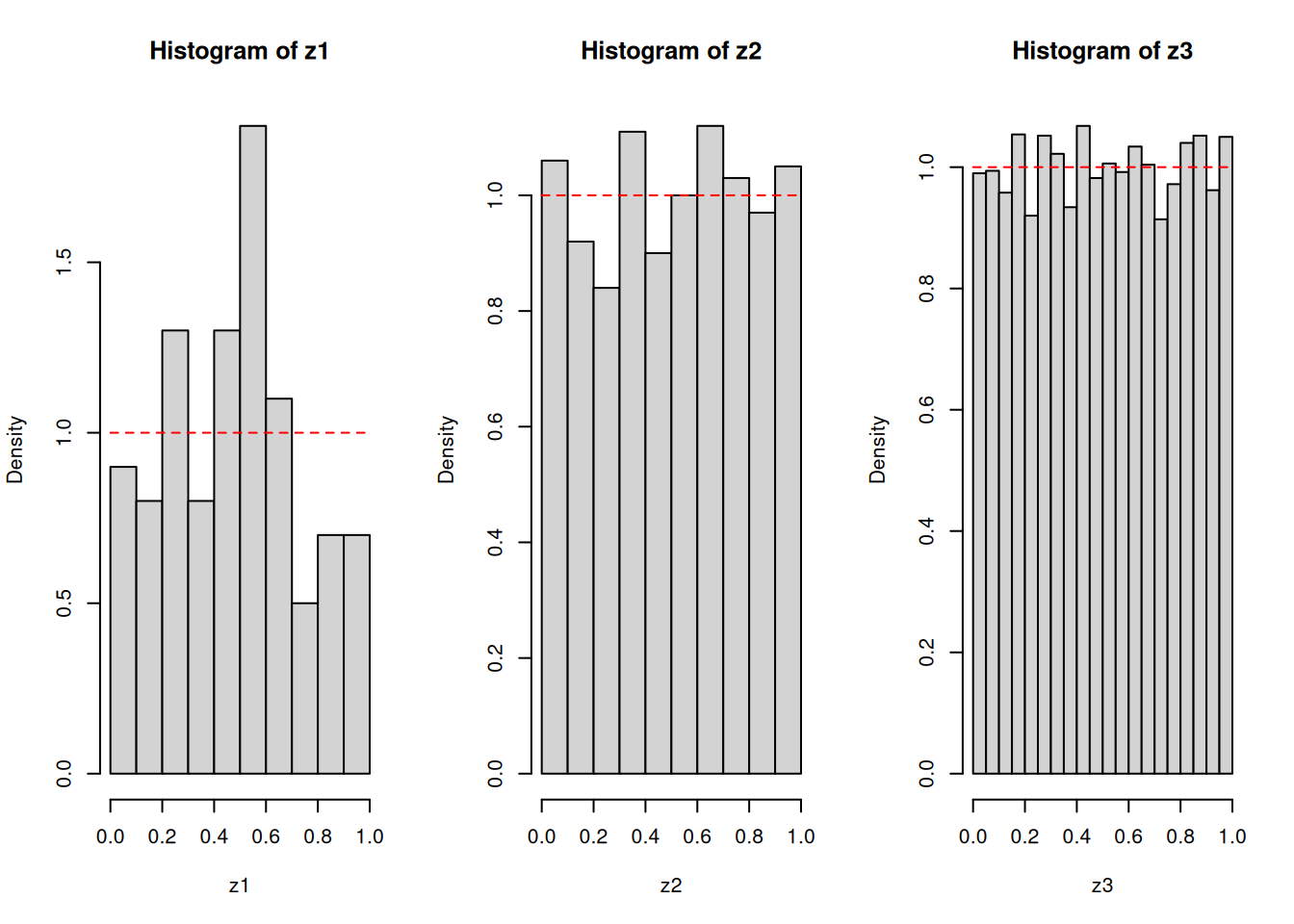
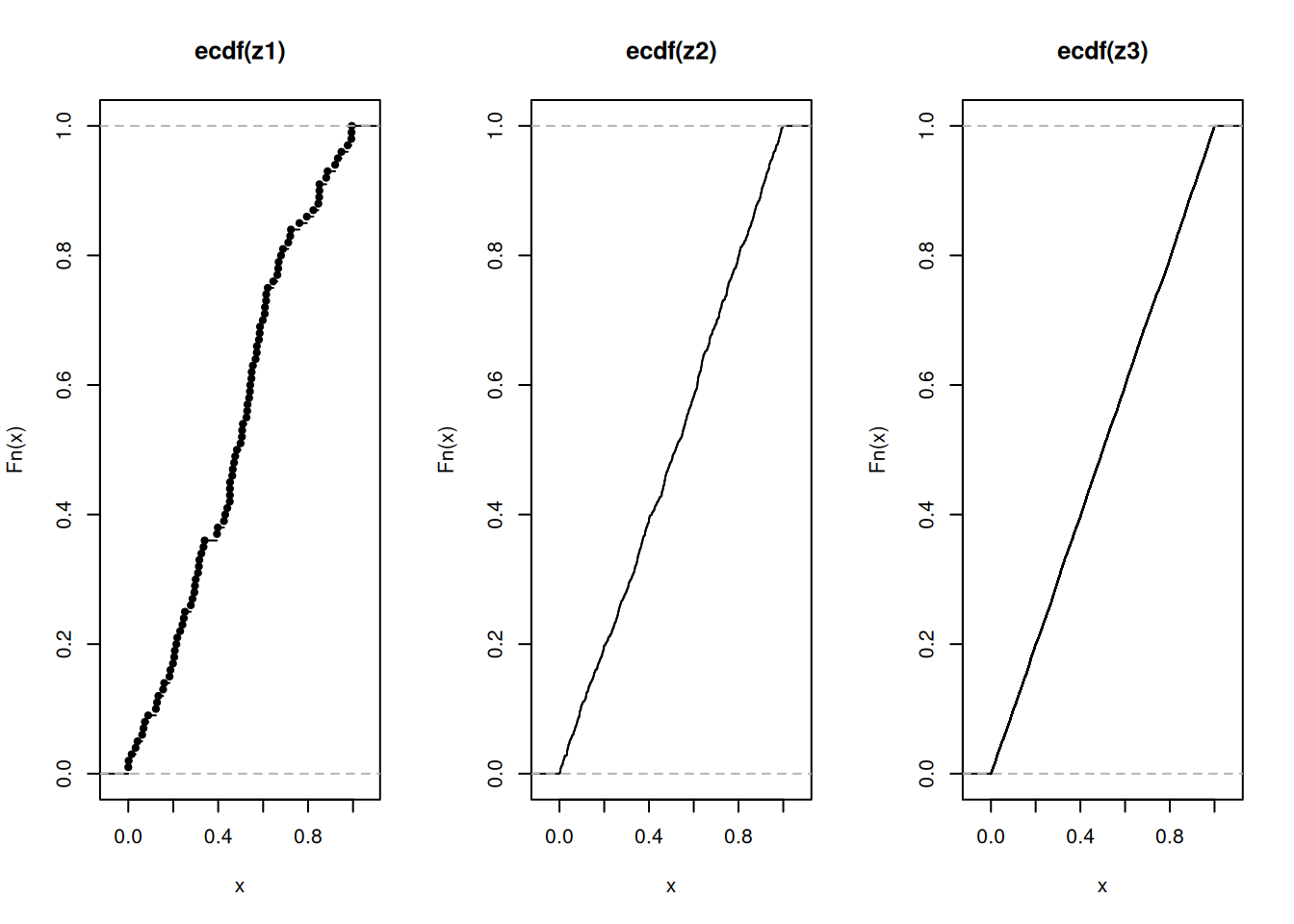
The preceding activity featured \(Z\sim U(0,1)\). We can actually use this distribution to draw “random” numbers which reflect the intuitive idea that any number is “equally likely” to be chosen from the interval \((0,1)\).
I will use the statistical software R to give you a sense of sampling from the uniform distribution on the interval \((0,1)\). It is not important to know all the details behind the code you see below, but it is important to know how the frequencies of the sampled numbers are behaving as you draw more and more numbers. Observe that the pdf, cdf, and the expected values can be thought of as “long-run” quantities, specifically, the “long-run” refers to drawing more and more numbers.
z1 <-runif(100)z2 <-runif(1000)z3 <-runif(10000)par(mfrow =c(1, 3))hist(z1, freq =FALSE)curve(1*(x >=0& x <=1), add =TRUE, lty =2, col ="red")hist(z2, freq =FALSE)curve(1*(x >=0& x <=1), add =TRUE, lty =2, col ="red")hist(z3, freq =FALSE)curve(1*(x >=0& x <=1), add =TRUE, lty =2, col ="red")
But, more importantly, it is possible to draw “random” numbers from any other continuous distribution with cdf \(G\) just based on “random” numbers from a \(U(0,1)\) distribution. The algorithm is as follows:
Draw “random” numbers from \(U(0,1)\).
Find the inverse of the cdf \(G\) and evaluate the it at each number drawn from the previous step. The resulting numbers are draws from the distribution with cdf \(G\).
This algorithm is supported by the following theorem:
Theorem 4.2 Let \(G\) be a cdf which is continuous and strictly increasing on the support of the distribution. Let \(Z\sim U(0,1)\) and \(X=G^{-1}\left(Z\right)\). Then \(X\) is an r.v. with cdf \(G\).
The proof is actually very simple for a result so useful. Let \(Z\sim U(0,1)\) and \(X=G^{-1}\left(Z\right)\). Let \(x\) be a given real number. We need to show that \(\mathbb{P}\left(X\leq x\right)\) matches \(G(x)\) for all \(x\).
First, observe that \(X=G^{-1}\left(Z\right)\). Therefore, \[\mathbb{P}\left(X\leq x\right)=\mathbb{P}\left(G^{-1}\left(Z\right)\leq x\right).\] Second, we can “undo” the inverse because \(G\) is strictly increasing. Therefore, \[\mathbb{P}\left(G^{-1}\left(Z\right)\leq x\right)=\mathbb{P}\left(Z\leq G(x)\right).\] Third, since \(Z\sim U(0,1)\), we can use the cdf of \(Z\) to evaluate \(\mathbb{P}\left(Z\leq G(x)\right)\). Therefore, \[\mathbb{P}\left(Z\leq G(x)\right)=G(x).\] Taking all the steps together, we obtain what needed to be shown: \[\mathbb{P}\left(X\leq x\right)=G(x).\] Therefore, the r.v. \(X\) will have a cdf which matches the desired cdf \(G\).
Activity
Return to our dart model. Recall that the cdf of \(D\) is given by Equation 4.4. How do we generate “random” numbers representing the distance of a dart from the center of the dart board? Consider the following code:
Explain why we have line 2 in light of Theorem 4.2. Try adjusting the number of darts to something larger, what do you expect to see from executing lines 4 to 6?
4.2.6 Exercises
Consider the logistic distribution with cdf \[F(x)=\dfrac{e^x}{1+e^x}\] for all real numbers \(x\).
Find the pdf. Verify that it is indeed a pdf.
Find \(\mathbb{P}\left(-2<X<2\right)\) in two ways – using the cdf and the pdf.
Write down an algorithm which will allows you to draw “random” numbers from the logistic distribution. Make sure to specify what the inverse cdf should be. If you can, create R code to implement this algorithm.
Find the expected value of \(X\).
Consider the Rayleigh distribution with cdf \[F(x)=1-e^{-x^2/2}\] for all real numbers \(x>0\).
Find the pdf. Verify that it is indeed a pdf.
Find \(\mathbb{P}\left(X>2\right)\) in two ways – using the cdf and the pdf.
Write down an algorithm which will allows you to draw “random” numbers from the logistic distribution. Make sure to specify what the inverse cdf should be. If you can, create R code to implement this algorithm.
Find the expected value of \(X\).
4.3 Numerical integration
4.3.1 Linearization and its improvements
Have you ever wondered how your calculator can produce a numeric approximation for complicated numbers like \(e\), \(\pi\) or \(\ln(2)\)? After all, the only operations a calculator can really perform are addition, subtraction, multiplication, and division, the operations that make up polynomials.
Preview Activity
This activity provides the first steps in understanding how this process works. Throughout the activity, let \(f(x) = e^x\).
Find the tangent line to \(f\) at \(x=0\) and use this linearization to approximate \(e\). That is, find a formula \(L(x)\) for the tangent line, and compute \(L(1)\), since \(L(1) \approx f(1) = e\).
The linearization of \(e^x\) does not provide a good approximation to \(e\) since 1 is not very close to 0. To obtain a better approximation, we alter our approach a bit. Instead of using a straight line to approximate \(e\), we put an appropriate bend in our estimating function to make it better fit the graph of \(e^x\) for \(x\) close to 0. With the linearization, we had both \(f(x)\) and \(f'(x)\) share the same value as the linearization at \(x=0\). We will now use a quadratic approximation \(P_2(x)\) to \(f(x) = e^x\) centered at \(x=0\) which has the property that \(P_2(0) = f(0)\), \(P'_2(0) = f'(0)\), and \(P''_2(0) = f''(0)\).
Let \(P_2(x) = 1+x+\frac{x^2}{2}\). Show that \(P_2(0) = f(0)\), \(P'_2(0) = f'(0)\), and \(P''_2(0) = f''(0)\). Then, use \(P_2(x)\) to approximate \(e\) by observing that \(P_2(1) \approx f(1)\).
We can continue approximating \(e\) with polynomials of larger degree whose higher derivatives agree with those of \(f\) at 0. This turns out to make the polynomials fit the graph of \(f\) better for more values of \(x\) around 0. For example, let \(P_3(x) = 1+x+\frac{x^2}{2}+\frac{x^3}{6}\). Show that \(P_3(0) = f(0)\), \(P'_3(0) = f'(0)\), \(P''_3(0) = f''(0)\), and \(P'''_3(0) = f'''(0)\). Use \(P_3(x)\) to approximate \(e\) in a way similar to how you did so with \(P_2(x)\) above.
Preview Activity
In this activity, we review and extend the process to find the “best” quadratic approximation to the exponential function \(e^x\) around the origin. Let \(f(x) = e^x\) throughout this activity.
Find a formula for \(P_1(x)\), the linearization of \(f(x)\) at \(x=0\). (We label this linearization \(P_1\) because it is a first degree polynomial approximation.) Recall that \(P_1(x)\) is a good approximation to \(f(x)\) for values of \(x\) close to \(0\). Plot \(f\) and \(P_1\) near \(x=0\) to illustrate this fact.
Since \(f(x) = e^x\) is not linear, the linear approximation eventually is not a very good one. To obtain better approximations, we want to develop a different approximation that “bends” to make it more closely fit the graph of \(f\) near \(x=0\). To do so, we add a quadratic term to \(P_1(x)\). In other words, we let \[\begin{equation*}
P_2(x) = P_1(x) + c_2x^2
\end{equation*}\] for some real number \(c_2\). We need to determine the value of \(c_2\) that makes the graph of \(P_2(x)\) best fit the graph of \(f(x)\) near \(x=0\).
Remember that \(P_1(x)\) was a good linear approximation to \(f(x)\) near \(0\); this is because \(P_1(0) = f(0)\) and \(P'_1(0) = f'(0)\). It is therefore reasonable to seek a value of \(c_2\) so that \[\begin{align*}
P_2(0) & = f(0)\text{,} & P'_2(0) & = f'(0)\text{,} & \text{and }P''_2(0) & = f''(0)\text{.}
\end{align*}\] Remember, we are letting \(P_2(x) = P_1(x) + c_2x^2\).
Calculate \(P_2(0)\) to show that \(P_2(0) = f(0)\).
Calculate \(P'_2(0)\) to show that \(P'_2(0) = f'(0)\).
Calculate \(P''_2(x)\). Then find a value for \(c_2\) so that \(P''_2(0) = f''(0)\).
Explain why the condition \(P''_2(0) = f''(0)\) will put an appropriate “bend” in the graph of \(P_2\) to make \(P_2\) fit the graph of \(f\) around \(x=0\).
4.3.2 Taylor polynomials
The two preview activities illustrate the first steps in the process of approximating functions with polynomials. Using this process we can approximate trigonometric, exponential, logarithmic, and other non-polynomial functions as closely as we like (for certain values of \(x\)) with polynomials. This is extraordinarily useful in that it allows us to calculate values of these functions to whatever precision we like using only the operations of addition, subtraction, multiplication, and division, which can be easily programmed in a computer.
We next extend the approach to arbitrary functions at arbitrary points. Let \(f\) be a function that has as many derivatives as we need at a point \(x=a\). Recall that \(P_1(x)\) is the tangent line to \(f\) at \((a,f(a))\) and is given by the formula \[\begin{equation*}
P_1(x) = f(a) + f'(a)(x-a)\text{.}
\end{equation*}\]\(P_1(x)\) is the linear approximation to \(f\) near \(a\) that has the same slope and function value as \(f\) at the point \(x = a\).
We next want to find a quadratic approximation \[\begin{equation*}
P_2(x) = P_1(x) + c_2(x-a)^2
\end{equation*}\] so that \(P_2(x)\) more closely models \(f(x)\) near \(x=a\). Consider the following calculations of the values and derivatives of \(P_2(x)\): \[\begin{align*}
P_2(x) & = P_1(x) + c_2(x-a)^2 & P_2(a) & = P_1(a) = f(a)\\
P'_2(x) & = P'_1(x) + 2c_2(x-a) & P'_2(a) & = P'_1(a) = f'(a)\\
P''_2(x) & = 2c_2 & P''_2(a) & = 2c_2\text{.}
\end{align*}\]
To make \(P_2(x)\) fit \(f(x)\) better than \(P_1(x)\), we want \(P_2(x)\) and \(f(x)\) to have the same concavity at \(x=a\), in addition to having the same slope and function value. That is, we want to have \[\begin{equation*}
P''_2(a) = f''(a)\text{.}
\end{equation*}\]
This implies that \[\begin{equation*}
2c_2 = f''(a)
\end{equation*}\] and thus \[\begin{equation*}
c_2 = \frac{f''(a)}{2}\text{.}
\end{equation*}\]
Therefore, the quadratic approximation \(P_2(x)\) to \(f\) centered at \(x=a\) is% \[\begin{equation*}
P_2(x) = f(a) + f'(a)(x-a) + \frac{f''(a)}{2!}(x-a)^2\text{.}
\end{equation*}\]
This approach extends naturally to polynomials of higher degree. We define polynomials \[\begin{align*}
P_3(x) & = P_2(x) + c_3(x-a)^3\text{,}\\
P_4(x) & = P_3(x) + c_4(x-a)^4\text{,}\\
P_5(x) & = P_4(x) + c_5(x-a)^5\text{,}
\end{align*}\] and in general \[\begin{equation*}
P_n(x) = P_{n-1}(x) + c_n(x-a)^n\text{.}
\end{equation*}\]
The defining property of these polynomials is that for each \(n\), \(P_n(x)\) and all its first \(n\) derivatives must agree with those of \(f\) at \(x = a\). In other words we require that \[\begin{equation*}
P^{(k)}_n(a) = f^{(k)}(a)
\end{equation*}\] for all \(k\) from 0 to \(n\).
To see the conditions under which this happens, suppose \[\begin{equation*}
P_n(x) = c_0 + c_1(x-a) + c_2(x-a)^2 + \cdots + c_n(x-a)^n\text{.}
\end{equation*}\]
So having \(P^{(k)}_n(a) = f^{(k)}(a)\) means that \(k!c_k = f^{(k)}(a)\) and therefore \[\begin{equation*}
c_k = \frac{f^{(k)}(a)}{k!}
\end{equation*}\] for each value of \(k\). Using this expression for \(c_k\), we have found the formula for the polynomial approximation of \(f\) that we seek. Such a polynomial is called a Taylor polynomial.
Definition 4.7 (Taylor polynomial) The \(n\)th order Taylor polynomial of \(f\) centered at \(x = a\) is given by \[\begin{align*}
P_n(x) =\mathstrut & f(a) + f'(a)(x-a) + \frac{f''(a)}{2!}(x-a)^2 + \cdots + \frac{f^{(n)}(a)}{n!}(x-a)^n\\
=\mathstrut & \sum_{k=0}^n \frac{f^{(k)}(a)}{k!}(x-a)^k\text{.}
\end{align*}\]
This degree \(n\) polynomial approximates \(f(x)\) near \(x=a\) and has the property that \(P_n^{(k)}(a) = f^{(k)}(a)\) for \(k = 0, 1, \ldots, n\).
Consider the following example. Determine the third order Taylor polynomial for \(f(x) = e^x\), as well as the general \(n\)th order Taylor polynomial for \(f\) centered at \(x=0\).
We know that \(f'(x) = e^x\) and so \(f''(x) = e^x\) and \(f'''(x) = e^x\). Thus, \[\begin{equation*}
f(0) = f'(0) = f''(0) = f'''(0) = 1\text{.}
\end{equation*}\]
So the third order Taylor polynomial of \(f(x) = e^x\) centered at \(x=0\) is \[\begin{align*}
P_3(x) & = f(0) + f'(0)(x-0) + \frac{f''(0)}{2!}(x-0)^2 + \frac{f'''(0)}{3!}(x-0)^3\\
& = 1 + x + \frac{x^2}{2} + \frac{x^3}{6}\text{.}
\end{align*}\]
In general, for the exponential function \(f\) we have \(f^{(k)}(x) = e^x\) for every positive integer \(k\). Thus, the \(k\)th term in the \(n\)th order Taylor polynomial for \(f(x)\) centered at \(x=0\) is \[\begin{equation*}
\frac{f^{(k)}(0)}{k!}(x-0)^k = \frac{1}{k!}x^k\text{.}
\end{equation*}\]
Therefore, the \(n\)th order Taylor polynomial for \(f(x) = e^x\) centered at \(x=0\) is \[\begin{equation*}
P_n(x) = 1+x+\frac{x^2}{2!} + \cdots + \frac{1}{n!}x^n = \sum_{k=0}^n \frac{x^k}{k!}\text{.}
\end{equation*}\]
Activity
Let \(f(x) = \frac{1}{1-x}\).
Calculate the first four derivatives of \(f(x)\) at \(x=0\). Then find the fourth order Taylor polynomial \(P_4(x)\) for \(\frac{1}{1-x}\) centered at \(0\).
Based on your results from the previous part, determine a general formula for \(f^{(k)}(0)\).
4.3.3 Trapezoid rule
We now develop numerical integration formulas for \(\displaystyle\int_a^b f(x)\,dx\) if the only information you have are the endpoints and the function values at the endpoints. Let \(f(a)\) and \(f(b)\) be those function values.
One possible way is to use the 1st order Taylor polynomial about \(a\) as a starting point, i.e. \[\int_a^b f(x)\,dx \approx \int_a^b P_1(x)\,dx.\] But \[P_1(x)=f(a)+f^\prime(a)(x-a)\] so that \[\begin{eqnarray*}\int_a^b P_1(x)\,dx &=& \int_a^b \left[f(a)+f^\prime(a)(x-a)\right]\,dx \\ &=& f(a)(b-a)+f^\prime(a) \frac{(b-a)^2}{2}\end{eqnarray*} \tag{4.5}\]
The issue is that we do not have information about \(f^\prime(a)\). We would have to replace it with an expression connected to the information we have available.
We can indirectly recover \(f^\prime(a)\) when we evaluate \(P_1(x)\) at \(x=b\). Observe that \[P_1(b)=f(a)+f^\prime(a)(b-a).\] Next, \(f(b)\) is approximately \(P_1(b)\), so that \[\begin{eqnarray*} f(b) &\approx& P_1(b) = f(a)+f^\prime(a)(b-a) \\ \Rightarrow \frac{f(b)-f(a)}{b-a} &\approx& f^\prime(a) \end{eqnarray*} \tag{4.6}\] Substituting Equation 4.6 into Equation 4.5, we obtain \[\begin{eqnarray*}\int_a^b P_1(x)\,dx &=& f(a)(b-a)+f^\prime(a) \frac{(b-a)^2}{2} \\ &\approx & f(a)(b-a)+\frac{f(b)-f(a)}{b-a}\cdot \frac{(b-a)^2}{2} \\
&=& \frac{1}{2}\left[f(a)+f(b)\right](b-a)\end{eqnarray*}\] Putting everything together, we have a first step towards developing the trapezoid rule. To summarize, we now have an approximation of \(\displaystyle\int_a^b f(x)\,dx\) only knowing the endpoints \(a\) and \(b\) along with the function values at those endpoints \(f(a)\) and \(f(b)\), i.e., \[\int_a^b f(x)\,dx\approx \frac{1}{2}\left[f(a)+f(b)\right](b-a) \tag{4.7}\]
We now extend Equation 4.7 by repeatedly applying its underlying idea over \(n\) equally spaced subintervals of \([a,b]\). We let \(h=(b-a)/n\). So, we have the following equally spaced subintervals \([a, a+h], [a+h, a+2h], \ldots, [a+(n-1)h, b]\). Now, apply Equation 4.7 to each subinterval and add all of the approximated areas together to obtain \[\begin{eqnarray*}\int_a^b f(x)\,dx &=& \int_a^{a+h}f(x)\,dx+\int_{a+h}^{a+2h}f(x)\,dx+\cdots+\int_{a+(n-1)h}^b f(x)\,dx \\ &\approx& \frac{1}{2}\left[f(a)+f(a+h)\right]h \\ && +\frac{1}{2}\left[f(a+h)+f(a+2h)\right]h \\ && + \frac{1}{2}\left[f(a+2h)+f(a+3h)\right]h \\ && + \cdots \\ && +\frac{1}{2}\left[f(a+(n-1)h)+f(b)\right]h \\ &=& \frac{h}{2}\left[f(a)+2\sum_{i=1}^{n-1} f(a+ih)+f(b)\right]\end{eqnarray*} \tag{4.8}\]
Equation 4.8 is the trapezoid rule used to approximate the definite integral \(\displaystyle\int_a^b f(x)\,dx\) where the only information we need to know are the points \(a, a+h, a+2h, \ldots, a+(n-1)h, b\) and the function \(f\) evaluated at these points.
4.3.4 Simpson’s rule
The numerical integration formula called Simpson’s rule follows the same arguments as how we obtained the trapezoid rule. The key differences are:
The information you have are the endpoints a, b, the midpoint \((a+b)/2\) and the function values at these three points. Let \(f(a)\), \(f((a+b)/2)\), and \(f(b)\) be those function values.
We use a second-order Taylor polynomial \(P_2(x)\) about the midpoint.
We use \(P_2(x)\) to approximate \(f(x)\), so that \[\int_a^b f(x)\,dx \approx \int_a^b P_2(x)\,dx.\] Based on Item 2, we have \[P_2(x) = f\left(\frac{a+b}{2}\right)+f^\prime\left(\frac{a+b}{2}\right)\left(x-\frac{a+b}{2}\right)+\frac{1}{2}f^{\prime\prime}\left(\frac{a+b}{2}\right)\left(x-\frac{a+b}{2}\right)^2.\] Therefore, \[\begin{eqnarray*}\int_a^b P_2(x)\,dx &=& f\left(\frac{a+b}{2}\right)(b-a) \\ && +f^\prime\left(\frac{a+b}{2}\right)\int_a^b \left(x-\frac{a+b}{2}\right)\,dx \\ && +\frac{1}{2}f^{\prime\prime}\left(\frac{a+b}{2}\right)\int_a^b\left(x-\frac{a+b}{2}\right)^2 \,dx \\
&=& f\left(\frac{a+b}{2}\right)(b-a) \\ && +f^\prime\left(\frac{a+b}{2}\right) \cdot 0 \\ && + \frac{1}{2}f^{\prime\prime}\left(\frac{a+b}{2}\right) \cdot \frac{2}{3}\left(\frac{b-a}{2}\right)^3 \\ &=& f\left(\frac{a+b}{2}\right)(b-a) + f^{\prime\prime}\left(\frac{a+b}{2}\right) \frac{(b-a)^3}{24}. \end{eqnarray*}\] This time, the issue is that we do not have information about \(\displaystyle f^{\prime\prime}\left(\frac{a+b}{2}\right)\). We would have to replace it with an expression connected to the information we have available in Item 1.
We compute \(P_2(a)\) and \(P_2(b)\) to make some progress. We now have \[\begin{eqnarray*} P_2(a) &=& f\left(\frac{a+b}{2}\right)+f^\prime\left(\frac{a+b}{2}\right)\frac{b-a}{2}+\frac{1}{2}f^{\prime\prime}\left(\frac{a+b}{2}\right)\left(\frac{b-a}{2}\right)^2 \\ P_2(b) &=& f\left(\frac{a+b}{2}\right)+f^\prime\left(\frac{a+b}{2}\right)\frac{a-b}{2}+\frac{1}{2}f^{\prime\prime}\left(\frac{a+b}{2}\right)\left(\frac{a-b}{2}\right)^2 \end{eqnarray*}\] Adding these two equations together, we have \[P_2(a)+P_2(b)=2f\left(\frac{a+b}{2}\right)+f^{\prime\prime}\left(\frac{a+b}{2}\right) \left(\frac{b-a}{2}\right)^2.\] Next, \(f(b)\) is approximately \(P_2(b)\) and \(f(a)\) is approximately \(P_2(a)\). We can now recover \(\displaystyle f^{\prime\prime}\left(\frac{a+b}{2}\right)\) using the only available information as described in Item 1: \[f^{\prime\prime}\left(\frac{a+b}{2}\right)\approx\dfrac{f(a)-2f\left(\dfrac{a+b}{2}\right) +f(b)}{\left(\dfrac{b-a}{2}\right)^2}.\]
Putting everything together, we have a first step towards developing Simpson’s rule. To summarize, we now have an approximation of \(\displaystyle\int_a^b f(x)\,dx\) only knowing the endpoints \(a\) and \(b\), the midpoint \((a+b)/2\), and the function values at these three points \(f(a)\), \(f(b)\), and \(f\left(\dfrac{a+b}{2}\right)\), i.e., \[\int_a^b f(x)\,dx\approx \frac{1}{6}\left[f(a)+4f\left(\dfrac{a+b}{2}\right)+f(b)\right](b-a) \tag{4.9}\]
We now extend Equation 4.9 by repeatedly applying its underlying idea over \(2n\) (instead of \(n\)) equally spaced subintervals of \([a,b]\). We let \(h=(b-a)/(2n)\). So, we have the following equally spaced subintervals \([a, a+2h], [a+2h, a+4h], \ldots, [a+(2n-2)h, b]\). Now, apply Equation 4.9 to each subinterval and add all of the approximated areas together to obtain \[\begin{eqnarray*}\int_a^b f(x)\,dx &=& \int_a^{a+2h}f(x)\,dx+\int_{a+2h}^{a+4h}f(x)\,dx+\cdots+\int_{a+(2n-2)h}^b f(x)\,dx \\ &\approx& \frac{1}{6}\left[f(a)+4f\left(a+h\right)+f(a+2h)\right](2h) \\ && +\frac{1}{6}\left[f(a+2h)+4f\left(a+3h\right)+f(a+4th)\right](2h) \\ && + \cdots \\ && + \frac{1}{6}\left[f(a+(2n-2)h)+4f\left(a+(2n-1)h\right)+f(b)\right](2h) \\ &=& \frac{h}{3}\left[f(a)+4\sum_{\mathrm{odd}\ i} f(a+ih)+2\sum_{\mathrm{even}\ i} f(a+ih)+f(b)\right]\end{eqnarray*} \tag{4.10}\]
Equation 4.10 is Simpson’s rule used to approximate the definite integral \(\displaystyle\int_a^b f(x)\,dx\) where the only information we need to know are the points \(a, a+h, a+2h, \ldots, a+(2n-1)h, b\) and the function \(f\) evaluated at these points.
4.4 Digging deeper
The applications presented only scratch the surface of what you can now do armed with just Chapter 1, Chapter 2, and Chapter 3. I end with some pointers to other possibilities for further exploration.
Our bank account application applies to continuous future income streams and these future income streams could represent dividends paid out to stockholders. It is possible to modify our activities to this setting and derive a way to value to stock of a company. This stock valuation method is called the Gordon dividend discount model.
Writing down expressions for the deadweight loss apply to other settings where a distortion is introduced. We can look into the impact of tariffs, quotas, and taxes, to name a few.
Our application to the Solow growth model can be made more complicated by allowing for technological progress in the aggregate production function. It is also possible to allow for the accumulation of human rather than just physical capital in the economy. These modifications require further studies in linear algebra and systems of differential equations.
You will see more applications related to probability and statistics in future major courses. But you have been exposed to a class of results summarizing the “long-run” behavior of random variables. These results are called law of large numbers. We mostly focused on relative frequencies and sample averages. To dig deeper, it may be good to look at the long-run behavior of quantities like the sample variance and the sample standard deviation.
We did not really show whether the trapezoid rule or Simpson’s rule will be preferable. To compare them, we need to be more specific about the approximation errors introduced by using the Taylor polynomials and the replacement of the derivatives by approximate differences. Digging deeper into these require further study about approximation errors.
In your first course in calculus, you have already been exposed to functions of more than one variable and a particular function class is called homogeneous functions. In economics, the function \(f\) is typically assumed to be homogeneous of degree one.↩︎
Intuitively, there is a sudden turn at that point when you graph Equation 4.4.↩︎