1 Motivating the need for integral calculus
1.1 To recover information about a function from its derivative
In this section, we try to answer the following questions:
If we know the velocity of a moving body at every point in a given interval, can we determine the distance the object has traveled on that given time interval?
How is the problem of finding distance traveled related to finding the area under a certain curve?
What does it mean to antidifferentiate a function and why is this process relevant to finding distance traveled?
We are contemplating the reverse situation, where we know the derivative of a function, \(f'\), and try to deduce information about \(f\). We will focus our attention on this problem: if we know the instantaneous rate of change of a function, can we find the function itself? We start with a more specific question: if we know the instantaneous velocity of an object moving along a straight line path, can we find its corresponding position function?
Preview Activity
Suppose that a person is taking a walk along a long straight path and walks at a constant rate of 3 miles per hour.
- On the left-hand axes provided in Figure 1.1, sketch a labeled graph of the velocity function \(v(t) = 3\).

Note that while the scale on the two sets of axes is the same, the units on the right-hand axes differ from those on the left. The right-hand axes will be used in question (d).
How far did the person travel during the two hours? How is this distance related to the area of a certain region under the graph of \(y = v(t)\)?
Find an algebraic formula, \(s(t)\), for the position of the person at time \(t\), assuming that \(s(0) = 0\). Explain your thinking.
On the right-hand axes provided in Figure 1.1, sketch a labeled graph of the position function \(y = s(t)\).
For what values of \(t\) is the position function \(s\) increasing? Explain why this is the case using relevant information about the velocity function \(v\).
1.1.1 Area under the graph of the velocity function
In the previous Preview Activity, we learned that when the velocity of a moving object’s velocity is constant (and positive), the area under the velocity curve over an interval of time tells us the distance the object traveled.

The left-hand graph of Figure 1.2 shows the velocity of an object moving at 2 miles per hour over the time interval \([1,1.5]\). The area \(A_1\) of the shaded region under \(y = v(t)\) on \([1,1.5]\) is
\[A_1= 2 \, \frac{\text{miles} }{\text{hour} } \cdot \frac{1}{2} \, \text{hours} = 1 \, \text{mile}\text{.}\]
This result is simply the fact that distance equals rate times time, provided the rate is constant. Thus, if \(v(t)\) is constant on the interval \([a,b]\), the distance traveled on \([a,b]\) is equal to the area \(A\) given by
\[A = v(a) (b-a) = v(a) \Delta t\text{,}\]
where \(\Delta t\) is the change in \(t\) over the interval. (Since the velocity is constant, we can use any value of \(v(t)\) on the interval \([a,b]\), we simply chose \(v(a)\), the value at the interval’s left endpoint.)
The situation is more complicated when the velocity function is not constant. But on relatively small intervals where \(v(t)\) does not vary much, we can use the area principle to estimate the distance traveled. The graph at right in Figure 1.2 shows a non-constant velocity function. On the interval \([1,1.5]\), the velocity varies from \(v(1) = 2.5\) down to \(v(1.5) \approx 2.1\). One estimate for the distance traveled is the area of the pictured rectangle,
\[A_2 = v(1) \Delta t = 2.5 \, \frac{\text{miles} }{\text{hour} } \cdot \frac{1}{2} \, \text{hours} = 1.25 \, \text{miles}\text{.}\]
Note that because \(v\) is decreasing on \([1,1.5]\), \(A_2 = 1.25\) is an over-estimate of the actual distance traveled.
To estimate the area under this non-constant velocity function on a wider interval, say \([0,3]\), one rectangle will not give a good approximation. Instead, we could use the six rectangles pictured in Figure 1.3, find the area of each rectangle, and add up the total. Obviously there are choices to make and issues to understand: How many rectangles should we use? Where should we evaluate the function to decide the rectangle’s height? Can we find the exact area under any non-constant curve?

We will study these questions and more in what follows; for now it suffices to observe that the simple idea of the area of a rectangle gives us a powerful tool for estimating distance traveled from a velocity function, as well as for estimating the area under an arbitrary curve.
For the ideas just described to work, we definitely need a way to link distance (or the position function) and velocity. Fortunately, velocity is a technical term and there are two notions of velocity.
For an object moving with position function \(s(t)\), the average velocity of the object on the interval from \(t = a\) to \(t = b\), denoted \(AV_{[a,b]}\), is given by the formula \[\begin{equation*} AV_{[a,b]} = \frac{s(b)-s(a)}{b-a}\text{.} \end{equation*}\]
The average velocity on \([a,b]\) can be viewed geometrically as the slope of the line between the points \((a,s(a))\) and \((b,s(b))\) on the graph of \(y = s(t)\), as shown in Figure 1.4.

Given a moving object whose position at time \(t\) is given by a function \(s\), the average velocity of the object on the time interval \([a,b]\) is given by \(AV_{[a,b]} = \frac{s(b) - s(a)}{b-a}\). Viewing the interval \([a,b]\) as having the form \([a,a+h]\), we equivalently compute average velocity by the formula \(AV_{[a,a+h]} = \frac{s(a+h) - s(a)}{h}\).
We find the instantaneous velocity of a moving object at a fixed time by taking the limit of average velocities of the object over shorter and shorter time intervals containing the time of interest.
Activity
Suppose that a person is walking in such a way that her velocity varies slightly according to the information given in Table 1.1 and graph given in Figure 1.5.
| \(t\) | \(v(t)\) |
|---|---|
| 0.00 | 1.500 |
| 0.25 | 1.789 |
| 0.50 | 1.938 |
| 0.75 | 1.992 |
| 1.00 | 2.000 |
| 1.25 | 2.008 |
| 1.50 | 2.063 |
| 1.75 | 2.211 |
| 2.00 | 2.500 |

Using the grid, graph, and given data appropriately, estimate the distance traveled by the walker during the two hour interval from \(t = 0\) to \(t = 2\). You should use time intervals of width \(\Delta t = 0.5\), choosing a way to use the function consistently to determine the height of each rectangle in order to approximate distance traveled.
How could you get a better approximation of the distance traveled on \([0,2]\)? Explain, and then find this new estimate.
Now suppose that you know that \(v\) is given by \(v(t) = 0.5t^3-1.5t^2+1.5t+1.5\). Can you try finding a formula for \(s\)?
Based on your work in (c), what is the value of \(s(2) - s(0)\)? What is the meaning of this quantity?
1.1.2 Two approaches: area and antidifferentiation
When the velocity of a moving object is positive, the object’s position is always increasing. (We will soon consider situations where velocity is negative; for now, we focus on the situation where velocity is always positive.) We have established that whenever \(v\) is constant on an interval, the exact distance traveled is the area under the velocity curve. When \(v\) is not constant, we can estimate the total distance traveled by finding the areas of rectangles that approximate the area under the velocity curve.
Thus, we see that finding the area between a curve and the horizontal axis is an important exercise: besides being an interesting geometric question, if the curve gives the velocity of a moving object, the area under the curve tells us the exact distance traveled on an interval. We can estimate this area if we have a graph or a table of values for the velocity function.
In the previous Activity, we encountered an alternate approach to finding the distance traveled. If \(y = v(t)\) is a formula for the instantaneous velocity of a moving object, then \(v\) must be the derivative of the object’s position function, \(s\). If we can find a formula for \(s(t)\) from the formula for \(v(t)\), we will know the position of the object at time \(t\), and the change in position over a particular time interval tells us the distance traveled on that interval.
For a simple example, consider the situation from the Preview Activity, where a person is walking along a straight line with velocity function \(v(t) = 3\) mph.

On the left-hand graph of the velocity function in Figure 1.6, we see the relationship between area and distance traveled,
\[ A= 3 \, \frac{\text{miles} }{\text{hour} } \cdot 1.25 \, \text{hours} = 3.75 \, \text{miles}\text{.}\]
In addition, we observe that if \(s(t) = 3t\), then \(s'(t) = 3\), so \(s(t) = 3t\) is the position function whose derivative is the given velocity function, \(v(t) = 3\). The respective locations of the person at times \(t = 0.25\) and \(t = 1.5\) are \(s(1.5) = 4.5\) and \(s(0.25) = 0.75\), and therefore
\[ s(1.5) - s(0.25) = 4.5 - 0.75 = 3.75 \ \text{miles}\text{.}\]
This is the person’s change in position on \([0.25,1.5]\), which is precisely the distance traveled.
For now, observe that if we know a formula for a velocity function \(v\), it can be very helpful to find a function \(s\) that satisfies \(s' = v\). We say that \(s\) is an antiderivative of \(v\). More generally, we have the following formal definition.
Definition 1.1 (Antiderivative) If \(g\) and \(G\) are functions such that \(G' = g\), we say that \(G\) is an antiderivative of \(g\).
For example, if \(g(x) = 3x^2 + 2x\), \(G(x) = x^3 + x^2\) is an antiderivative of \(g\), because \(G'(x) = g(x)\). Note that we say an antiderivative of \(g\) rather than the antiderivative of \(g\), because \(H(x) = x^3 + x^2 + 5\) is also a function whose derivative is \(g\), and thus \(H\) is another antiderivative of \(g\).
Activity
A ball is tossed vertically in such a way that its velocity function is given by \(v(t) = 32 - 32t\), where \(t\) is measured in seconds and \(v\) in feet per second. Assume that this function is valid for \(0 \le t \le 2\).
For what values of \(t\) is the velocity of the ball positive? What does this tell you about the motion of the ball on this interval of time values?
Find an antiderivative, \(s\), of \(v\) that satisfies \(s(0) = 0\).
Compute the value of \(s(1) - s(\frac{1}{2})\). What is the meaning of the value you find?
Using the graph of \(y = v(t)\) provided in Figure 1.7, find the exact area of the region between the velocity curve and the \(t\)-axis between \(t = \frac{1}{2}\) and \(t = 1\). What is the meaning of the value you find?

- What is the value of \(s(2) - s(0)\)? What does this result tell you about the flight of the ball? How is this value connected to the provided graph of \(y = v(t)\)? Explain.
1.1.3 Exercises
- Two cars start at the same time and travel in the same direction along a straight road. The figure below gives the velocity, \(v\) (in km/hr), of each car as a function of time (in hr). The velocity of car A is given by the solid, blue curve, and the velocity of car B by dashed, red curve. Which car attains the larger maximum velocity? Which stops first? Which travels farther?

The velocity function is \(v(t) = t^2 - 3 t + 2\) for a particle moving along a line. Find the displacement (net distance covered) of the particle during the time interval \([-2,5]\).
A toy rocket is launched vertically from the ground on a day with no wind. The rocket’s vertical velocity at time \(t\) (in seconds) is given by \(v(t)= 500-32t\) feet/sec.
- At what time after the rocket is launched does the rocket’s velocity equal zero? Call this time value \(a\). What happens to the rocket at \(t = a\)?
- Find the value of the total area enclosed by \(y = v(t)\) and the \(t\)-axis on the interval \(0 \le t \le a\). What does this area represent in terms of the physical setting of the problem?
- Find an antiderivative \(s\) of the function \(v\). That is, find a function \(s\) such that \(s'(t) = v(t)\).
- Compute the value of \(s(a) - s(0)\). What does this number represent in terms of the physical setting of the problem?
- Compute \(s(5) - s(1)\). What does this number tell you about the rocket’s flight?
Filters at a water treatment plant become dirtier over time and thus become less effective; they are replaced every 30 days. During one 30-day period, the rate at which pollution passes through the filters into a nearby lake (in units of particulate matter per day) is measured every 6 days and is given in the following table. The time \(t\) is measured in days since the filters were replaced.
- Plot the given data on a set of axes with time on the horizontal axis and the rate of pollution on the vertical axis.
- Explain why the amount of pollution that entered the lake during this 30-day period would be given exactly by the area bounded by \(y = p(t)\) and the \(t\)-axis on the time interval \([0,30]\).
- Estimate the total amount of pollution entering the lake during this 30-day period. Carefully explain how you determined your estimate.
| Day, \(t\) | 0 | 6 | 12 | 18 | 24 | 30 |
| Rate of pollution in units per day, \(p(t)\) | 7 | 8 | 10 | 13 | 18 | 35 |
1.2 To solve differential equations
In this section, we try to answer the following questions:
- What is a differential equation and what kinds of information can it tell us?
- What do we mean by a solution to a differential equation?
We have seen that a function’s derivative tells us the rate at which the function is changing. For example, an object’s velocity tells us the rate of change of that object’s position. How can we determine how much the position changes over that time interval? If we know where the object is at the beginning of that interval, we actually have enough information to predict where it will be at the end of the interval.
We introduce the concept of differential equations. A differential equation is an equation that provides a description of a function’s derivative, which means that it tells us the function’s rate of change. Using this information, we would like to learn as much as possible about the function itself. Ideally we would like to have an algebraic description of the function. As we’ll see, this may be too much to ask in some situations, but we will still be able to make accurate approximations.
Preview Activity
The position of a moving object is given by the function \(s(t)\), where \(s\) is measured in feet and \(t\) in seconds. We determine that the velocity is \(v(t) = 4t + 1\) feet per second.
- How much does the position change over the time interval \([0,4]\)?
- Does this give you enough information to determine \(s(4)\), the position at time \(t=4\)? If so, what is \(s(4)\)? If not, what additional information would you need to know to determine \(s(4)\)?
- Suppose you are told that the object’s initial position \(s(0) = 7\). Determine \(s(2)\), the object’s position 2 seconds later.
- If you are told instead that the object’s initial position is \(s(0) = 3\), what is \(s(2)\)?
- If we only know the velocity \(v(t)=4t+1\), is it possible that the object’s position at all times is \(s(t) = 2t^2 + t - 4\)? Explain how you know.
- Are there other possibilities for \(s(t)\)? If so, what are they?
- If, in addition to knowing the velocity function is \(v(t) = 4t+1\), we know the initial position \(s(0)\), how many possibilities are there for \(s(t)\)?
1.2.1 What is a differential equation?
A differential equation is an equation that describes the derivative, or derivatives, of a function that is unknown to us. For instance, the equation
\[\frac{dy}{dx} = 2y\]
describes the derivative of a function \(y(x)\) that is unknown to us.
As many important examples of differential equations involve quantities that change in time, the independent variable in our discussion will frequently be time \(t\). In the preview activity, we considered the differential equation
\[\frac{ds}{dt} = 4t + 1\text{.}\]
Knowing the velocity and the starting position of a moving object, we were able to find its position at any later time.
Because differential equations describe the derivative of a function, they give us information about how that function changes. Our goal will be to use this information to predict the value of the function in the future; in this way, differential equations provide us with something like a crystal ball.
Differential equations arise frequently in our every day world. For instance, you may hear a bank advertising:
Your money will grow at a 3% annual interest rate with us.
This innocuous statement is really a differential equation. Let’s translate: \(A(t)\) will be amount of money you have in your account at time \(t\). The rate at which your money grows is the derivative \(dA/dt\), and we are told that this rate is \(0.03 A\). This leads to the differential equation
\[\frac{dA}{dt} = 0.03 A\text{.}\]
This differential equation has a slightly different feel than the previous equation \(\frac{ds}{dt} = 4t+1\). In the earlier example, the rate of change depends only on the independent variable \(t\), and we may find \(s(t)\) by finding an antiderivative to the velocity function \(4t+1\). In the banking example, however, the rate of change depends on the dependent variable \(A\), so we’ll need some new techniques in order to find \(A(t)\).1
Activity
Express the following statements as differential equations. In each case, you will need to introduce notation to describe the important quantities in the statement so be sure to clearly state what your notation means.
- The population of a town grows continuously at an annual rate of 1.25%.
- A radioactive sample loses mass at a rate of 5.6% of its mass every day.
- You have a bank account that continuously earns 4% interest every year. At the same time, you withdraw money continually from the account at the rate of 1000 dollars per year.
- A cup of hot chocolate is sitting in a 70\(^\circ\) F room. The temperature of the hot chocolate cools continuously by 10% of the difference between the hot chocolate’s temperature and the room temperature every minute.
- A can of cold soda is sitting in a 70\(^\circ\) F room. The temperature of the soda warms continuously at the rate of 10% of the difference between the soda’s temperature and the room’s temperature every minute.
1.2.2 Solving a differential equation
A differential equation describes the derivative, or derivatives, of a function that is unknown to us. By a solution to a differential equation, we mean simply a function that satisfies this description.
For instance, the first differential equation we looked at is
\[\frac{ds}{dt} = 4t+1\text{,}\]
which describes an unknown function \(s(t)\). We may check that \(s(t) = 2t^2+t\) is a solution because it satisfies this description. Notice that \(s(t) = 2t^2+t+4\) is also a solution.
If we have a candidate for a solution, it is straightforward to check whether it is a solution or not. Before we demonstrate, however, let’s consider the same issue in a simpler context. Suppose we are given the equation \(2x^2 - 2x = 2x+6\) and asked whether \(x=3\) is a solution. To answer this question, we could rewrite the variable \(x\) in the equation with the symbol \(\square\):
\[2\square^2 - 2\square = 2\square + 6\text{.}\]
To determine whether \(x=3\) is a solution, we can investigate the value of each side of the equation separately when the value \(3\) is placed in \(\square\) and see if indeed the two resulting values are equal. Doing so, we observe that
\[2\square^2 - 2\square = 2\cdot3^2 - 2\cdot3 = 12\text{,}\]
and
\[2\square + 6 = 2\cdot3 + 6 = 12\text{.}\]
Therefore, \(x=3\) is indeed a solution.
We will do the same thing with differential equations. Consider the differential equation2
\[\frac{dv}{dt} = 1.5 - 0.5v, \ \text{or} \frac{d\square}{dt} = 1.5 - 0.5\square\text{.}\]
Let’s ask whether \(v(t) = 3 - 2e^{-0.5t}\) is a solution. Using this formula for \(v\), observe first that
\[\frac{dv}{dt} = \frac{d\square}{dt} = \frac{d}{dt}[3 - 2e^{-0.5t}] = -2e^{-0.5t} \cdot (-0.5) = e^{-0.5t}\]
and
\[1.5 - 0.5v = 1.5 - 0.5\square= 1.5 - 0.5(3 - 2e^{-0.5t}) = 1.5 - 1.5 + e^{-0.5t} = e^{-0.5t}\text{.}\]
Since \(\frac{dv}{dt}\) and \(1.5 - 0.5v\) agree for all values of \(t\) when \(v = 3-2e^{-0.5t}\), we have indeed found a solution to the differential equation.
Activity
Consider the differential equation
\[\frac{dv}{dt} = 1.5 - 0.5v\text{.}\]
Which of the following functions are solutions of this differential equation?
- \(v(t) = 1.5t - 0.25t^2\)
- \(v(t) = 3 + 2e^{-0.5t}\)
- \(v(t) = 3\)
- \(v(t) = 3 + Ce^{-0.5t}\) where \(C\) is any constant.
The previous activity shows us something interesting. Notice that the differential equation has infinitely many solutions, which are parametrized by the constant \(C\) in \(v(t) = 3+Ce^{-0.5t}\). In Figure 1.8, we see the graphs of these solutions for a few values of \(C\), as labeled.

Notice that the value of \(C\) is connected to the initial value of \(v(0)\), since \(v(0) = 3+C\). In other words, while the differential equation describes how \(v\) changes over time as a function of the \(v\) itself, this is not enough information to determine the velocity uniquely: we also need to know the initial value \(v(0)\). For this reason, differential equations will typically have infinitely many solutions, one corresponding to each initial value.
We have seen the phenomenon described earlier: given the velocity of a moving object \(v(t)\), we cannot uniquely determine the object’s position function \(s(t)\) unless we also know its initial position \(s(0)\).
If we are given a differential equation and an initial value for the unknown function, we say that we have an initial value problem. For instance,
\[\frac{dv}{dt} = 1.5-0.5v, \ v(0) = 0.5\]
is an initial value problem. In this problem, we know the value of \(v\) at one time and we know how \(v\) is changing. Consequently, there should be exactly one function \(v\) that satisfies the initial value problem.
This demonstrates the following important general property of initial value problems.
Initial value problems that are “well behaved” have exactly one solution, which exists in some interval around the initial point.
We won’t worry about what “well behaved” means – it is a technical condition that will be satisfied by all the differential equations we consider.
To close this section, we note that differential equations may be classified based on certain characteristics they may possess. You may see many different types of differential equations in a later course in differential equations. For now, we would like to introduce a few terms that are used to describe differential equations.
A first-order differential equation is one in which only the first derivative of the function occurs. For this reason,
\[\frac{dv}{dt} = 1.5-0.5v\]
is a first-order equation while
\[\frac{d^2 y}{dt^2} = -10y\]
is a second-order equation.
A differential equation is autonomous if the independent variable does not appear in the description of the derivative. For instance,
\[\frac{dv}{dt} = 1.5-0.5v\]
is autonomous because the description of the derivative \(dv/dt\) does not depend on time. The equation
\[\frac{dy}{dt} = 1.5t - 0.5y\text{,}\]
however, is not autonomous.
1.2.3 Qualitative behavior of solutions to differential equations
In this subsection, we ask the following questions:
- What is a slope field?
- How can we use a slope field to obtain qualitative information about the solutions of a differential equation?
- What are stable and unstable equilibrium solutions of an autonomous differential equation?
In your course in differential calculus, you have used the tangent line to the graph of a function \(f\) at a point \(a\) to approximate the values of \(f\) near \(a\). The usefulness of this approximation is that we need to know very little about the function; armed with only the value \(f(a)\) and the derivative \(f'(a)\), we may find the equation of the tangent line and the approximation
\[f(x) \approx f(a) + f'(a)(x-a)\text{.}\]
Remember that a first-order differential equation gives us information about the derivative of an unknown function. Since the derivative at a point tells us the slope of the tangent line at this point, a differential equation gives us crucial information about the tangent lines to the graph of a solution. We will use this information about the tangent lines to create a slope field for the differential equation, which enables us to sketch solutions to initial value problems. Our aim will be to understand the solutions qualitatively. That is, we would like to understand the basic nature of solutions, such as their long-range behavior, without precisely determining the value of a solution at a particular point.
Preview Activity
Let’s consider the initial value problem
\[\frac{dy}{dt} = t - 2, \ \ y(0) = 1\text{.}\]
- Use the differential equation to find the slope of the tangent line to the solution \(y(t)\) at \(t=0\). Then use the initial value to find the equation of the tangent line at \(t=0\). Sketch this tangent line over the interval \(-0.25 \leq t \leq 0.25\) on the axes provided in Figure 1.9.

- Also shown in Figure 1.9 are the tangent lines to the solution \(y(t)\) at the points \(t=1, 2\), and \(3\) (we will see how to find these later). Use the graph to measure the slope of each tangent line and verify that each agrees with the value specified by the differential equation.
- Using these tangent lines as a guide, sketch a graph of the solution \(y(t)\) over the interval \(0\leq t\leq 3\) so that the lines are tangent to the graph of \(y(t)\).
- Attempt to find \(y(t)\), the solution to this initial value problem.
- Graph the solution you found in (d) on the axes provided, and compare it to the sketch you made using the tangent lines.
1.2.3.1 Slope fields
The previous Preview Activity shows that we can sketch the solution to an initial value problem if we know an appropriate collection of tangent lines. We can use the differential equation to find the slope of the tangent line at any point of interest, and hence plot such a collection.
Let’s continue looking at the differential equation \(\frac{dy}{dt} = t-2\). If \(t=0\), this equation says that \(dy/dt = 0-2=-2\). Note that this value holds regardless of the value of \(y\). We will therefore sketch tangent lines for several values of \(y\) and \(t=0\) with a slope of \(-2\), as shown in Figure 1.10.


Let’s continue in the same way: if \(t=1\), the differential equation tells us that \(dy/dt = 1-2=-1\), and this holds regardless of the value of \(y\). We now sketch tangent lines for several values of \(y\) and \(t=1\) with a slope of \(-1\) in Figure 1.11.
Similarly, we see that when \(t=2\), \(dy/dt = 0\) and when \(t=3\), \(dy/dt=1\). We may therefore add to our growing collection of tangent line plots to achieve Figure 1.12.


In Figure 1.12, we begin to see the solutions to the differential equation emerge. For the sake of even greater clarity, we add more tangent lines to provide the more complete picture shown at right in Figure 1.13.
Figure 1.13 is called a slope field for the differential equation. It allows us to sketch solutions just as we did in the preview activity. We can begin with the initial value \(y(0) = 1\) and start sketching the solution by following the tangent line. Whenever the solution passes through a point at which a tangent line is drawn, that line is tangent to the solution. This principle leads us to the sequence of images in


In fact, we can draw solutions for any initial value. Figure 1.15 shows solutions for several different initial values for \(y(0)\).

Just as we did for the equation \(\frac{dy}{dt} = t-2\), we can construct a slope field for any differential equation of interest. The slope field provides us with visual information about how we expect solutions to the differential equation to behave.
Activity
Consider the autonomous differential equation
\[\frac{dy}{dt} = -\frac{1}{2}(y - 4)\text{.}\]
- Make a plot of \(\frac{dy}{dt}\) versus \(y\) on the axes provided in Figure 1.16. Looking at the graph, for what values of \(y\) does \(y\) increase and for what values of \(y\) does \(y\) decrease?


- Next, sketch the slope field for this differential equation on the axes provided in Figure 1.17.
- Use your work in (b) to sketch (on the same axes in Figure 1.17) solutions that satisfy \(y(0) = 0\), \(y(0) = 2\), \(y(0) = 4\) and \(y(0) = 6\).
- Verify that \(y(t) = 4 + 2e^{-t/2}\) is a solution to the given differential equation with the initial value \(y(0) = 6\). Compare its graph to the one you sketched in (c).
- What is special about the solution where \(y(0) = 4\)?
1.2.3.2 Equilibrium solutions and stability
As our work in the previous activity demonstrates, first-order autonomous equations may have solutions that are constant. These are simple to detect by inspecting the differential equation \(dy/dt = f(y)\): constant solutions necessarily have a zero derivative, so \(dy/dt = 0 = f(y)\).
For example, in the previous activity, we considered the equation \(\frac{dy}{dt} = f(y)=-\frac{1}{2}(y-4)\). Constant solutions are found by setting \(f(y) = -\frac{1}{2}(y-4) = 0\), which we immediately see implies that \(y = 4\).
Values of \(y\) for which \(f(y) = 0\) in an autonomous differential equation \(\frac{dy}{dt} = f(y)\) are called equilibrium solutions of the differential equation.
Activity
Consider the autonomous differential equation
\[\frac{dy}{dt} = -\frac{1}{2}y(y-4)\text{.}\]
- Make a plot of \(\frac{dy}{dt}\) versus \(y\) on the axes provided in Figure 1.18. Looking at the graph, for what values of \(y\) does \(y\) increase and for what values of \(y\) does \(y\) decrease?


Identify any equilibrium solutions of the given differential equation.
Now sketch the slope field for the given differential equation on the axes provided in Figure 1.19.
Sketch the solutions to the given differential equation that correspond to initial values \(y(0)=-1, 0, 1, \ldots, 5\).
An equilibrium solution \(\overline{y}\) is called stable if nearby solutions converge to \(\overline{y}\). This means that if the initial condition varies slightly from \(\overline{y}\), then \(\lim_{t\to\infty}y(t) = \overline{y}\). In contrast, an equilibrium solution \(\overline{y}\) is called unstable if nearby solutions are pushed away from \(\overline{y}\). Using your work above, classify the equilibrium solutions you found in (b) as either stable or unstable.
Suppose that \(y(t)\) describes the population of a species of living organisms and that the initial value \(y(0)\) is positive. What can you say about the eventual fate of this population?
Now consider a general autonomous differential equation of the form \(dy/dt = f(y)\). Remember that an equilibrium solution \(\overline{y}\) satisfies \(f(\overline{y}) = 0\). If we graph \(dy/dt = f(y)\) as a function of \(y\), for which of the differential equations represented in Figure 1.20 and Figure 1.21 is \(\overline{y}\) a stable equilibrium and for which is \(\overline{y}\) unstable? Why?


1.2.4 Exercises
- Let \(A\) and \(k\) be positive constants. Which of the given functions is a solution to \(\frac{dy}{dt}=-k(y+A)\)?
- \(\displaystyle y = -A + C e^{-kt}\)
- \(\displaystyle y = A + C e^{-kt}\)
- \(\displaystyle y = -A + C e^{kt}\)
- \(\displaystyle y = A^{-1} + C e^{Akt}\)
- \(\displaystyle y = A + C e^{kt}\)
- \(\displaystyle y = A^{-1} + C e^{-Akt}\)
- Suppose that \(T(t)\) represents the temperature of a cup of coffee set out in a room, where \(T\) is expressed in degrees Fahrenheit and \(t\) in minutes. A physical principle known as Newton’s Law of Cooling tells us that \[\frac{dT}{dt}= -\frac1{15}T+5\text{.}\]
- Suppose that \(T(0)=105\). What does the differential equation give us for the value of \(\frac{dT}{dt}\vert_{T=105}\)? Explain in a complete sentence the meaning of these two facts.
- Is \(T\) increasing or decreasing at \(t=0\)?
- What is the approximate temperature at \(t=1\)?
- On the graph below, make a plot of \(dT/dt\) as a function of \(T\).

- For which values of \(T\) does \(T\) increase? For which values of \(T\) does \(T\) decrease?
- What do you think is the temperature of the room? Explain your thinking.
- Verify that \(T(t) = 75 + 30e^{-t/15}\) is the solution to the differential equation with initial value \(T(0) = 105\). What happens to this solution after a long time?
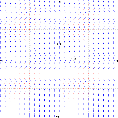
- Consider the slope field below for a differential equation. Use the graph to find the equilibrium solutions and, if possible, determine their stability.
Suppose that the population of a particular species is described by the function \(P(t)\), where \(P\) is expressed in millions. Suppose further that the population’s rate of change is governed by the differential equation \[\frac{dP}{dt} = f(P)\] where \(f(P)\) is the function graphed on the right.

- For which values of the population \(P\) does the population increase?
- For which values of the population \(P\) does the population decrease?
- If \(P(0) = 3\), how will the population change in time?
- If the initial population satisfies \(0< P(0)< 1\), what will happen to the population after a very long time?
- If the initial population satisfies \(1< P(0)< 3\), what will happen to the population after a very long time?
- If the initial population satisfies \(3< P(0)\), what will happen to the population after a very long time?
- This model for a population’s growth is sometimes called “growth with a carrying capacity and a critical threshold”. Explain why this is an appropriate name.
- Sketch a slope field for this differential equation. You do not have enough information to determine the actual slopes, but you should have enough information to determine where slopes are positive, negative, zero, large, or small, and hence determine the qualitative behavior of solutions.
- Sketch some solutions to this differential equation when the initial population \(P(0) > 0\).
- Identify any equilibrium solutions to the differential equation and classify them as stable or unstable.
- If \(P(0) > 1\), what is the eventual fate of the species? if \(P(0) < 1\)?
You are given the differential equation \(x'(t) = -(x-1)(x+1)(x+4)(x+5)\). List the constant (or equilibrium) solutions to this differential equation in increasing order and indicate whether or not these equilibria are stable or unstable.
The population of a species of fish in a lake is \(P(t)\) where \(P\) is measured in thousands of fish and \(t\) is measured in months. The growth of the population is described by the differential equation \[\begin{equation*} \frac{dP}{dt} = f(P) = P(6-P)\text{.} \end{equation*}\]
- Sketch a graph of \(f(P) = P(6-P)\) and use it to determine the equilibrium solutions and whether they are stable or unstable. Write a complete sentence that describes the long-term behavior of the fish population.
- Suppose now that the owners of the lake allow fishers to remove 1000 fish from the lake every month (remember that \(P(t)\) is measured in thousands of fish). Modify the differential equation to take this into account. Sketch the new graph of \(dP/dt\) versus \(P\). Determine the new equilibrium solutions and decide whether they are stable or unstable.
- Given the situation in part (ii), give a description of the long-term behavior of the fish population.
- Suppose that fishermen remove \(h\) thousand fish per month. How is the differential equation modified?
- What is the largest number of fish that can be removed per month without eliminating the fish population? If fish are removed at this maximum rate, what is the eventual population of fish?
1.3 Summary of main points
If we know the velocity of a moving body at every point in a given interval and the velocity is positive throughout, we can estimate the object’s distance traveled and in some circumstances determine this value exactly.
In particular, when velocity is positive on an interval, we can find the total distance traveled by finding the area under the velocity curve and above the \(t\)-axis on the given time interval. We may only be able to estimate this area, depending on the shape of the velocity curve.
An antiderivative of a function \(f\) is a new function \(F\) whose derivative is \(f\). That is, \(F\) is an antiderivative of \(f\) provided that \(F' = f\). In the context of velocity and position, if we know a velocity function \(v\), an antiderivative of \(v\) is a position function \(s\) that satisfies \(s' = v\). If \(v\) is positive on a given interval, say \([a,b]\), then the change in position, \(s(b) - s(a)\), measures the distance the moving object traveled on \([a,b]\).
A differential equation is simply an equation that describes the derivative(s) of an unknown function.
Physical principles, as well as some everyday situations, often describe how a quantity changes, which lead to differential equations.
A solution to a differential equation is a function whose derivatives satisfy the equation’s description. Differential equations typically have infinitely many solutions, parametrized by the initial values.
A slope field is a plot created by graphing the tangent lines of many different solutions to a differential equation.
Once we have a slope field, we may sketch the graph of solutions by drawing a curve that is always tangent to the lines in the slope field.
Autonomous differential equations sometimes have constant solutions that we call equilibrium solutions. These may be classified as stable or unstable, depending on the behavior of nearby solutions.