2 The connections among area, antiderivatives, and solutions to differential equations
2.1 Euler’s method
In this section, we answer the following questions:
- What is Euler’s method and how can we use it to approximate the solution to an initial value problem?
- How is Euler’s method ultimately connected to areas under a curve?
In Section 1.2.3, we saw how a slope field can be used to sketch solutions to a differential equation. In particular, the slope field is a plot of a large collection of tangent lines to a large number of solutions of the differential equation, and we sketch a single solution by simply following these tangent lines. With a little more thought, we can use this same idea to approximate numerically the solutions of a differential equation.
Preview Activity
Consider the initial value problem \[\begin{equation*} \frac{dy}{dt} = \frac12 (y + 1), \ y(0) = 0\text{.} \end{equation*}\] a. Use the differential equation to find the slope of the tangent line to the solution \(y(t)\) at \(t=0\). Then use the given initial value to find the equation of the tangent line at \(t=0\).
- Sketch the tangent line on the axes provided in Figure 2.1 on the interval \(0\leq t\leq 2\) and use it to approximate \(y(2)\), the value of the solution at \(t=2\).

- Assuming that your approximation for \(y(2)\) is the actual value of \(y(2)\), use the differential equation to find the slope of the tangent line to \(y(t)\) at \(t=2\). Then, write the equation of the tangent line at \(t=2\).
- Add a sketch of this tangent line on the interval \(2\leq t\leq 4\) to your plot Figure 2.1; use this new tangent line to approximate \(y(4)\), the value of the solution at \(t=4\).
- Repeat the same step to find an approximation for \(y(6)\).
2.1.1 The algorithm behind Euler’s method
The previous activity demonstrates an algorithm known as Euler’s1 Method, which generates a numerical approximation to the solution of an initial value problem. In this algorithm, we will approximate the solution by taking horizontal steps of a fixed size that we denote by \(\Delta t\).
Before explaining the algorithm in detail, let’s remember how we compute the slope of a line: the slope is the ratio of the vertical change to the horizontal change, as shown in Figure 2.2.

In other words, \(m = \frac{\Delta y}{\Delta t}\). Solving for \(\Delta y\), we see that the vertical change is the product of the slope and the horizontal change, or \[\begin{equation*} \Delta y = m\Delta t\text{.} \end{equation*}\]
Now, suppose that we would like to solve the initial value problem \[\begin{equation*} \frac{dy}{dt} = t - y, \ y(0) = 1\text{.} \end{equation*}\]
There is an algorithm by which we can find an algebraic formula for the solution to this initial value problem, and we can check that this solution is \(y(t) = t -1 + 2e^{-t}\). But we are instead interested in generating an approximate solution by creating a sequence of points \((t_i, y_i)\), where \(y_i\approx y(t_i)\). For this first example, we choose \(\Delta t = 0.2\).
Since we know that \(y(0) = 1\), we will take the initial point to be \((t_0,y_0) = (0,1)\) and move horizontally by \(\Delta t = 0.2\) to the point \((t_1,y_1)\). Thus, \(t_1=t_0+\Delta t = 0.2\). Now, the differential equation tells us that the slope of the tangent line at this point is \[\begin{equation*} m=\frac{dy}{dt}\bigg\vert_{(0,1)} = 0-1 = -1\text{,} \end{equation*}\] so to move along the tangent line by taking a horizontal step of size \(\Delta t=0.2\), we must also move vertically by \[\begin{equation*} \Delta y = m\Delta t = -1\cdot 0.2 = -0.2\text{.} \end{equation*}\] We then have the approximation \(y(0.2) \approx y_1= y_0 + \Delta y = 1 - 0.2 = 0.8\). At this point, we have executed one step of Euler’s method, as seen graphically in Figure 2.3.

Now we repeat this process: at \((t_1,y_1) = (0.2,0.8)\), the differential equation tells us that the slope is \[\begin{equation*} m=\frac{dy}{dt}\bigg\vert_{(0.2,0.8)} = 0.2-0.8 = -0.6\text{.} \end{equation*}\]
If we move forward horizontally by \(\Delta t\) to \(t_2=t_1+\Delta = 0.4\), we must move vertically by \[\begin{equation*} \Delta y = -0.6\cdot0.2 = -0.12\text{.} \end{equation*}\] We consequently arrive at \(y_2=y_1+\Delta y = 0.8-0.12 = 0.68\), which gives \(y(0.4)\approx 0.68\). Now we have completed the second step of Euler’s method, as shown in Figure 2.4.

If we continue in this way, we may generate the points \((t_i, y_i)\) shown in Figure 2.5. Because we can find a formula for the actual solution \(y(t)\) to this differential equation, we can graph \(y(t)\) and compare it to the points generated by Euler’s method, as shown in Figure 2.6.


Because we need to generate a large number of points \((t_i,y_i)\), it is convenient to organize the implementation of Euler’s method in a table as shown. We begin with the given initial data.
| \(t_i\) | \(y_i\) | \(dy/dt\) | \(\Delta y\) |
|---|---|---|---|
| \(0.0000\) | \(1.0000\) |
From here, we compute the slope of the tangent line \(m=dy/dt\) using the formula for \(dy/dt\) from the differential equation, and then we find \(\Delta y\), the change in \(y\), using the rule \(\Delta y = m\Delta t\).
| \(t_i\) | \(y_i\) | \(dy/dt\) | \(\Delta y\) |
|---|---|---|---|
| \(0.0000\) | \(1.0000\) | \(-1.0000\) | \(-0.2000\) |
Next, we increase \(t_i\) by \(\Delta t\) and \(y_i\) by \(\Delta y\) to get
| \(t_i\) | \(y_i\) | \(dy/dt\) | \(\Delta y\) |
|---|---|---|---|
| \(0.0000\) | \(1.0000\) | \(-1.0000\) | \(-0.2000\) |
| \(0.2000\) | \(0.8000\) |
We continue the process for however many steps we decide, eventually generating a table like
| \(t_i\) | \(y_i\) | \(dy/dt\) | \(\Delta y\) |
|---|---|---|---|
| \(0.0000\) | \(1.0000\) | \(-1.0000\) | \(-0.2000\) |
| \(0.2000\) | \(0.8000\) | \(-0.6000\) | \(-0.1200\) |
| \(0.4000\) | \(0.6800\) | \(-0.2800\) | \(-0.0560\) |
| \(0.6000\) | \(0.6240\) | \(-0.240\) | \(-0.0048\) |
| \(0.8000\) | \(0.6192\) | \(0.1808\) | \(0.0362\) |
| \(1.0000\) | \(0.6554\) | \(0.3446\) | \(0.0689\) |
| \(1.2000\) | \(0.7243\) | \(0.4757\) | \(0.0951\) |
Since we are approximating the solutions to an initial value problem using tangent lines, we should expect that the error in the approximation will be smaller when the step size is smaller.
We do not explore the quantification of the approximation error. Instead, we note a result which will be left unproved here in the text. Let the approximations be denoted by \(\widehat{y}_{\Delta t}(\overline{t})\). If Euler’s method is used to approximate the solution to an initial value problem at a point \(\overline{t}\), then the error is proportional to \(\Delta t\). That is, \[\begin{equation*} y(\overline{t}) - \widehat{y}_{\Delta t}(\overline{t}) \approx K\Delta t \end{equation*}\] for some unknown constant of proportionality \(K\).
2.1.2 A connection to area
The tabular calculations you have seen so far when you apply Euler’s method may be reinterpreted in terms of areas. As a result, we have a connection between solutions of differential equations and the area under a curve. The next activity allows you to explore this idea.
Activity
Consider the initial value problem \[\begin{equation*} \frac{dy}{dt} = 2t, \ y(0) = 0 \end{equation*}\]
- Use Euler’s method with \(\Delta t = 0.2\) to approximate the solution at \(t_i = 0.2, 0.4, 0.6, 0.8\), and \(1.0\). Record your work in a tabular format with columns for \(t_i\), \(y_i\), \(dy/dt\), and \(\Delta y\), and sketch the points \((t_i, y_i)\) on the axes provided.
- Find the exact solution to the original initial value problem and use this function to find the error in your approximation at each one of the points \(t_i\).
- Explain how the value \(y_5\) generated by Euler’s method for this initial value problem coincides with a particular estimate of the area of the region bounded by \(t\)-axis, the curve \(g(t)=2t\), \(t=0\), and \(t=1\).
- How would your computations differ if the initial value was \(y(0) = 1\)? What does this mean about different solutions to this differential equation?
- How would your response to Item 3 differ if the initial value problem were \[\begin{equation*} \frac{dy}{dt} = -2t, \ y(0) = 0 \end{equation*}\] What do you think about the notion of area in this situation?
If you have worked through the activity, then you have explicitly gone through an argument as to why approximate solutions of differential equations may be given an area interpretation. In addition, as you make \(\Delta t\) smaller and smaller, the approximate solutions should approach the exact solution to the initial value problem. In some initial value problems like the previous activity, finding an exact solution is as simple as finding an antiderivative. Therefore, there is a strong connection among antiderivatives, area, and solutions of differential equations.2
In fact, we can also revisit our activities involving constant and non-constant velocity functions and cast them in terms of differential equations. We return to this context in the next section.
2.1.3 Exercises
- Consider the differential equation \(y'=-x-y\).
- Use Euler’s method with \(\Delta x=0.1\) to estimate \(y\) when \(x=1.4\) for the solution curve satisfying \(y(1)=1\).
- Use Euler’s method with \(\Delta x=0.1\) to estimate \(y\) when \(x=2.4\) for the solution curve satisfying \(y(1) = 0\).
- Consider the solution of the differential equation \(y' = -2 y\) passing through \(y(0) = 1\).
- Sketch the slope field for this differential equation, and sketch the solution passing through the point (0,1).
- Use Euler’s method with step size \(\Delta x=0.2\) to estimate the solution at \(x=0.2,0.4,\ldots,1\), using these to fill in the following table. Be sure not to round your answers at each step!
- Plot your estimated solution on your slope field. Compare the solution and the slope field. Is the estimated solution an over or under estimate for the actual solution?
- Check that \(y = e^{-2 x}\) is a solution to \(y' = -2 y\) with \(y(0) = 1\).
- Use Euler’s method to solve \[\begin{equation*}
\frac{dB}{dt}= 0.05 B
\end{equation*}\] with initial value \(B=800\) when \(t=0\)
- \(\Delta t = 1\) and 1 step: \(B(1) \approx ?\)
- \(\Delta t = 0.5\) and 2 steps: \(B(1) \approx ?\)
- \(\Delta t = 0.25\) and 4 steps: \(B(1) \approx ?\)
- Suppose \(B\) is the balance in a bank account earning interest. Be sure that you can explain why the result of your calculation in Item (a) is equivalent to compounding the interest once a year instead of continuously. Then interpret the result of your calculations in Items (b) and (c) in terms of compound interest.
- Consider the initial value problem \[\begin{equation*}
\frac{dy}{dt} = y, \ y(0) = 1\text{,}
\end{equation*}\] whose solution we can easily find. The question posed by this initial value problem is “what function do we know that is the same as its own derivative and has value 1 when \(t=0\)?” It is not hard to see that the solution is \(y(t) = e^t\).
- Verify that \(y(t) = e^t\) is the solution to the initial value problem.3
- Apply Euler’s method to approximate \(y(1) = e\) using \(\Delta t=0.2, 0.1, 0.5, 0.025\). Calculate the errors produced by Euler’s method. Plot the errors on the vertical axis and step size on the horizontal axis. Confirm, both numerically and graphically, that the error is roughly halved when \(\Delta t\) is halved.
- We have seen that the error in approximating the solution to an initial value problem is proportional to \(\Delta t\). That is, if \(\widehat{y}_{\Delta t}\left(\overline{t}\right)\) is the Euler’s method approximation to the solution to an initial value problem at \(\overline{t}\), then \[\begin{equation*}
y(\overline{t})-\widehat{y}_{\Delta t}\left(\overline{t}\right) \approx K\Delta t
\end{equation*}\] for some constant of proportionality \(K\). In this problem, we will see how to use this fact to improve our estimates, using an idea called accelerated convergence.
- We will create a new approximation by assuming the error is exactly proportional to \(\Delta t\), according to the formula \[\begin{equation*} y(\overline{t})-\widehat{y}_{\Delta t}\left(\overline{t}\right) =K\Delta t\text{.} \end{equation*}\] Using our earlier results from the initial value problem \(dy/dt = y\) and \(y(0)=1\) with \(\Delta t = 0.2\) and \(\Delta t = 0.1\), we have \[\begin{align*} y(1) - 2.4883 =\mathstrut & 0.2K\\ y(1) - 2.5937 =\mathstrut & 0.1K\text{.} \end{align*}\] This is a system of two linear equations in the unknowns \(y(1)\) and \(K\). Solve this system to find a new approximation for \(y(1)\). (You may remember that the exact value is \(y(1) = e = 2.71828\ldots\).)
- Use the other data, \(\widehat{y}_{0.05}\left(1\right) = 2.6533\) and \(\widehat{y}_{0.025}\left(1\right) = 2.6851\) to do similar work as in (a) to obtain another approximation. Which gives the better approximation? Why do you think this is?
- Let’s now study the initial value problem \[\begin{equation*} \frac{dy}{dt} = t-y, \ y(0) = 0\text{.} \end{equation*}\] Approximate \(y(0.3)\) by applying Euler’s method to find approximations \(\widehat{y}_{0.1}(0.3)\) and \(\widehat{y}_{0.05}(0.3)\). Now use the idea of accelerated convergence to obtain a better approximation. (For the sake of comparison, you want to note that the actual value is \(y(0.3) = 0.0408\).)
2.2 Riemann sums
In this section, we answer the following questions:
- How can we use a Riemann sum to estimate the area between a given curve and the horizontal axis over a particular interval?
- What are the differences among left, right, middle, and random Riemann sums?
- How can we write Riemann sums in an abbreviated form?
2.2.1 When the function is positive
When a moving body has a positive velocity function \(y = v(t)\) on a given interval \([a,b]\), the area under the curve over the interval gives the total distance the body travels on \([a,b]\). In a more general setting, we are also interested in finding the exact area bounded by \(y = f(x)\) on an interval \([a,b]\), regardless of the meaning or context of the function \(f\).
For now, we continue to focus on finding an accurate estimate of this area by using a sum of the areas of rectangles. Unless otherwise indicated, we assume that \(f\) is continuous and non-negative on \([a,b]\).
The first choice we make in such an approximation is the number of rectangles.

If we desire \(n\) rectangles of equal width to subdivide the interval \([a,b]\), then each rectangle must have width \(\Delta x = \frac{b-a}{n}\). We let \(x_0 = a\), \(x_n = b\), and define \(x_{i} = a + i\Delta x\), so that \(x_1 = x_0 + \Delta x\), \(x_2 = x_0 + 2 \Delta x\), and so on, as pictured in Figure 2.8.
We use each subinterval \([x_i, x_{i+1}]\) as the base of a rectangle, and next choose the height of the rectangle on that subinterval. There are three standard choices: we can use the left endpoint of each subinterval, the right endpoint of each subinterval, or the midpoint of each. We alluded to these options as early as in Section 1.1.1.
Consider an arbitrary positive function \(f\) on \([a,b]\) with the interval subdivided as shown in Figure 2.8, and choose to use left endpoints. Then on each interval \([x_{i}, x_{i+1}]\), the area of the rectangle formed is given by \[\begin{equation*} A_{i+1} = f(x_i) \cdot \Delta x\text{,} \end{equation*}\] as seen in Figure 2.9.

If we let \(L_n\) denote the sum of the areas of these rectangles, we see that \[\begin{align*} L_n =\mathstrut & A_1 + A_2 + \cdots + A_{i+1} + \cdots + A_n\\ =\mathstrut & f(x_0) \cdot \Delta x + f(x_1) \cdot \Delta x + \cdots + f(x_i) \cdot \Delta x + \cdots + f(x_{n-1}) \cdot \Delta x\text{.} \end{align*}\] The expression above would be sufficient. An alternative way of writing the expression is in the more compact sigma notation or summation notation.4 We have \[\begin{equation*} L_n = \sum_{i = 0}^{n-1} f(x_i) \Delta x\text{.} \end{equation*}\]
Note that since the index of summation begins at \(0\) and ends at \(n-1\), there are indeed \(n\) terms in this sum. We call \(L_n\) the left Riemann sum for the function \(f\) on the interval \([a,b]\).
To see how the Riemann sums for right endpoints and midpoints are constructed, we consider Figure 2.10.

For the sum with right endpoints, we see that the area of the rectangle on an arbitrary interval \([x_i, x_{i+1}]\) is given by \(B_{i+1} = f(x_{i+1}) \cdot \Delta x\), and that the sum of all such areas of rectangles is given by \[\begin{align*} R_n =\mathstrut & B_1 + B_2 + \cdots + B_{i+1} + \cdots + B_n\\ =\mathstrut & f(x_1) \cdot \Delta x + f(x_2) \cdot \Delta x + \cdots + f(x_{i+1}) \cdot \Delta x + \cdots + f(x_{n}) \cdot \Delta x\\ =\mathstrut & \sum_{i=1}^{n} f(x_i) \Delta x\text{.} \end{align*}\]
We call \(R_n\) the right Riemann sum for the function \(f\) on the interval \([a,b]\).
For the sum that uses midpoints, we introduce the notation \[\begin{equation*} \overline{x}_{i+1} = \frac{x_{i} + x_{i+1}}{2} \end{equation*}\] so that \(\overline{x}_{i+1}\) is the midpoint of the interval \([x_i, x_{i+1}]\). For instance, for the rectangle with area \(C_1\) in Figure 2.10, we now have \[\begin{equation*} C_1 = f(\overline{x}_1) \cdot \Delta x\text{.} \end{equation*}\]
Hence, the sum of all the areas of rectangles that use midpoints is \[\begin{align*} M_n =\mathstrut & C_1 + C_2 + \cdots + C_{i+1} + \cdots + C_n\\ =\mathstrut & f(\overline{x_1}) \cdot \Delta x + f(\overline{x_2}) \cdot \Delta x + \cdots + f(\overline{x}_{i+1}) \cdot \Delta x + \cdots + f(\overline{x}_{n}) \cdot \Delta x\\ =\mathstrut & \sum_{i=1}^{n} f(\overline{x}_i) \Delta x\text{,} \end{align*}\] and we say that \(M_n\) is the middle Riemann sum for \(f\) on \([a,b]\).
When \(f(x) \ge 0\) on \([a,b]\), each of the Riemann sums \(L_n\), \(R_n\), and \(M_n\) provides an estimate of the area under the curve \(y = f(x)\) over the interval \([a,b]\). We also recall that in the context of a nonnegative velocity function \(y = v(t)\), the corresponding Riemann sums approximate the distance traveled on \([a,b]\) by a moving object with velocity function \(v\).
There is a more general way to think of Riemann sums, and that is to allow any choice of where the function is evaluated to determine the rectangle heights. Rather than saying we’ll always choose left endpoints, or always choose midpoints, we simply say that a point \(x_{i+1}^*\) will be selected at random in the interval \([x_i, x_{i+1}]\) (so that \(x_i \le x_{i+1}^* \le x_{i+1}\)). The Riemann sum is then given by \[\begin{equation*} f(x_1^*) \cdot \Delta x + f(x_2^*) \cdot \Delta x + \cdots + f(x_{i+1}^*) \cdot \Delta x + \cdots + f(x_n^*) \cdot \Delta x = \sum_{i=1}^{n} f(x_i^*) \Delta x\text{.} \end{equation*}\]
In computations encountered in calculus, we most often use \(L_n\), \(R_n\), or \(M_n\), while the random Riemann sum is useful in theoretical discussions. However, there is a useful connection between the formation of a random Riemann sum and probability and statistical theory. We will explore this aspect later in a subsequent chapter.
In the following activity, we investigate several different Riemann sums for a particular velocity function.
Activity
Suppose that an object moving along a path has its velocity in feet per second at time \(t\) in seconds given by \(v(t) = \frac{2}{9}(t-3)^2 + 2\).
- Carefully sketch the region whose exact area will tell you the value of the distance the object traveled on the time interval \(2 \le t \le 5\).
- Estimate the distance traveled on \([2,5]\) by computing \(L_4\), \(R_4\), and \(M_4\).
- Does averaging \(L_4\) and \(R_4\) result in the same value as \(M_4\)? If not, what do you think the average of \(L_4\) and \(R_4\) measures?
- For this question, think about an arbitrary function \(f\), rather than the particular function \(v\) given above. If \(f\) is positive and increasing on \([a,b]\), will \(L_n\) over-estimate or under-estimate the exact area under \(f\) on \([a,b]\)? Will \(R_n\) over- or under-estimate the exact area under \(f\) on \([a,b]\)? Explain.
2.2.2 When the function is sometimes negative
For a Riemann sum such as \[\begin{equation*} L_n = \sum_{i=0}^{n-1} f(x_i) \Delta x\text{,} \end{equation*}\] we can of course compute the sum even when \(f\) takes on negative values. We know that when \(f\) is positive on \([a,b]\), a Riemann sum estimates the area bounded between \(f\) and the horizontal axis over the interval.

For the function pictured in the first graph of Figure 2.11, a left Riemann sum with 12 subintervals over \([a,d]\) is shown. The function is negative on the interval \(b \le x \le c\), so at the four left endpoints that fall in \([b,c]\), the terms \(f(x_i) \Delta x\) are negative. This means that those four terms in the Riemann sum produce an estimate of the opposite of the area bounded by \(y = f(x)\) and the horizontal axis on \([b,c]\).
In the middle graph of Figure 2.11, we see that by increasing the number of rectangles the approximation of the area (or the opposite of the area) bounded by the curve appears to improve.
In general, any Riemann sum of a continuous function \(f\) on an interval \([a,b]\) approximates the difference between the area that lies above the horizontal axis on \([a,b]\) and under \(f\) and the area that lies below the horizontal axis on \([a,b]\) and above \(f\). In the notation of Figure 2.11, we may say that
\[\begin{equation*} L_{24} \approx A_1 - A_2 + A_3\text{,} \end{equation*}\] where \(L_{24}\) is the left Riemann sum using 24 subintervals shown in the middle graph. \(A_1\) and \(A_3\) are the areas of the regions where \(f\) is positive, and \(A_2\) is the area where \(f\) is negative. We will call the quantity \(A_1 - A_2 + A_3\) the net signed area bounded by \(f\) over the interval \([a,d]\), where by the phrase “signed area” we indicate that we are attaching a minus sign to the areas of regions that fall below the horizontal axis.
Finally, we recall that if the function \(f\) represents the velocity of a moving object, the sum of the areas bounded by the curve tells us the total distance traveled over the relevant time interval, while the net signed area bounded by the curve computes the object’s change in position on the interval.
Activity
Suppose that an object moving along a path has its velocity \(v\) (in feet per second) at time \(t\) (in seconds) given by \[\begin{equation*} v(t) = \frac{1}{2}t^2 - 3t + \frac{7}{2}\text{.} \end{equation*}\]
- Compute \(M_5\), the middle Riemann sum, for \(v\) on the time interval \([1,5]\). Be sure to clearly identify the value of \(\Delta t\) as well as the locations of \(t_0\), \(t_1\), \(\cdots\), \(t_5\). In addition, provide a careful sketch of the function and the corresponding rectangles that are being used in the sum.
- Building on your work in Item 1, estimate the total change in position of the object on the interval \([1,5]\).
- Building on your work in Items 1 and 2, estimate the total distance traveled by the object on \([1,5]\).
- Use appropriate computing technology to compute \(M_{10}\) and \(M_{20}\). What exact value do you think the middle sum eventually approaches as \(n\) increases without bound? What does that number represent in the physical context of the overall problem?
2.2.3 Exercises
- Start from the graph of \(y = e^{x}\).
- Represent the left Riemann sum with \(n = 2\) approximating \(\int_{0}^{1}\,e^{x}\,dx\). Write out the terms of the sum, but do not evaluate it.
- Represent the right Riemann sum with \(n = 2\) approximating \(\int_{0}^{1}\,e^{x}\,dx\). Write out the terms of the sum, but do not evaluate it.
- Which sum is an overestimate? Which sum is an underestimate?
- Consider the function \(f(x) = 3x + 4\).
- Compute \(M_4\) for \(y=f(x)\) on the interval \([2,5]\). Be sure to clearly identify the value of \(\Delta x\), as well as the locations of \(x_0, x_1, \ldots, x_4\). Include a careful sketch of the function and the corresponding rectangles being used in the sum.
- Use a familiar geometric formula to determine the exact value of the area of the region bounded by \(y = f(x)\) and the \(x\)-axis on \([2,5]\).
- Explain why the values you computed in (a) and (b) turn out to be the same. Will this be true if we use a number different than \(n = 4\) and compute \(M_n\)? Will \(L_4\) or \(R_4\) have the same value as the exact area of the region found in (b)?
- Describe the collection of functions \(g\) for which it will always be the case that \(M_n\), regardless of the value of \(n\), gives the exact net signed area bounded between the function \(g\) and the \(x\)-axis on the interval \([a,b]\).
- Let \(S\) be the sum given by \[\begin{equation*}
S = ((1.4)^2 + 1) \cdot 0.4 + ((1.8)^2 + 1) \cdot 0.4 + ((2.2)^2 + 1) \cdot 0.4 + ((2.6)^2 + 1) \cdot 0.4 +((3.0)^2 + 1) \cdot 0.4\text{.}
\end{equation*}\]
- Assume that \(S\) is a right Riemann sum. For what function \(f\) and what interval \([a,b]\) is \(S\) this function’s Riemann sum? Why?
- How does your answer to (a) change if \(S\) is a left Riemann sum? a middle Riemann sum?
- Suppose that \(S\) really is a right Riemann sum. What is geometric quantity does \(S\) approximate?
- Use sigma notation to write a new sum \(R\) that is the right Riemann sum for the same function, but that uses twice as many subintervals as \(S\).
- The rate at which pollution escapes a scrubbing process at a manufacturing plant increases over time as filters and other technologies become less effective. For this particular example, assume that the rate of pollution (in tons per week) is given by the function \(r\) that is pictured in Figure 2.12.
- Use the graph to estimate the value of \(M_4\) on the interval \([0,4]\).
- What is the meaning of \(M_4\) in terms of the pollution discharged by the plant?
- Suppose that \(r(t) = 0.5 e^{0.5t}\). Use this formula for \(r\) to compute \(L_5\) on \([0,4]\).
- Determine an upper bound on the total amount of pollution that can escape the plant during the pictured four week time period that is accurate within an error of at most one ton of pollution.

2.3 The definite integral
In this section, we answer the following questions:
- What is the definition of the definite integral of a function \(f\) over the interval \([a,b]\)?
- What does the definite integral measure exactly, and what are some of the key properties of the definite integral?
In Figure 2.11, we see evidence that increasing the number of rectangles in a Riemann sum improves the accuracy of the approximation of the net signed area bounded by the given function. This motivates an approach to define the limiting value of a Riemann sum.
2.3.1 The definition of the definite integral
We have built some intuition that as the number of rectangles got larger and larger, the values of \(L_n\), \(M_n\), and \(R_n\) all grew closer and closer to the same value. It turns out that this occurs for any continuous function on an interval \([a,b]\), and also for a Riemann sum using any point \(x_{i+1}^*\) in the interval \([x_i, x_{i+1}]\). Thus, as we let \(n \to \infty\), it doesn’t really matter where we choose to evaluate the function within a given subinterval, because \[\begin{equation*} \lim_{n \to \infty} L_n = \lim_{n \to \infty} R_n = \lim_{n \to \infty} M_n = \lim_{n \to \infty} \sum_{i=1}^{n} f(x_i^*) \Delta x\text{.} \end{equation*}\] That these limits always exist (and share the same value) when \(f\) is continuous5 allows us to make the following definition.
Definition 2.1 (Definite Integral) The definite integral of a continuous function \(f\) on the interval \([a,b]\), denoted \(\int_a^b f(x) \, dx\), is the real number given by \[\begin{equation*} \int_a^b f(x) \, dx = \lim_{n \to \infty} \sum_{i=1}^{n} f(x_i^*) \Delta x\text{,} \end{equation*}\] where \(\Delta x = \frac{b-a}{n}\), \(x_i = a + i\Delta x\) (for \(i = 0, \ldots, n\)), and \(x_i^*\) satisfies \(x_{i-1} \leq x_i^* \leq x_i\) (for \(i = 1, \ldots, n\)).
We call the symbol \(\int\) the integral sign, the values \(a\) and \(b\) the limits of integration, and the function \(f\) the integrand. The process of determining the real number \(\int_a^b f(x) \, dx\) is called evaluating the definite integral. While there are several different interpretations of the definite integral, for now the most important is that \(\int_a^b f(x) \, dx\) measures the net signed area bounded by \(y = f(x)\) and the horizontal axis on the interval \([a,b]\).
For example, if \(f\) is the function pictured in Figure 2.13, and \(A_1\), \(A_2\), and \(A_3\) are the exact areas bounded by \(f\) and the horizontal axis on the respective intervals \([a,b]\), \([b,c]\), and \([c,d]\), then \[\begin{gather*} \int_a^b f(x) \, dx = A_1, \ \int_b^c f(x) \, dx = -A_2,\\ \int_c^d f(x) \, dx = A_3,\\ \text{ and } \int_a^d f(x) \, dx = A_1 - A_2 + A_3\text{.} \end{gather*}\]

We can also use definite integrals to express the change in position and the distance traveled by a moving object. If \(v\) is a velocity function on an interval \([a,b]\), then the change in position of the object, \(s(b) - s(a)\), is given by \[\begin{equation*} s(b) - s(a) = \int_a^b v(t) \, dt\text{.} \end{equation*}\]
If the velocity function is nonnegative on \([a,b]\), then \(\int_a^b v(t) \,dt\) tells us the distance the object traveled. If the velocity is sometimes negative on \([a,b]\), we can use definite integrals to find the areas bounded by the function on each interval where \(v\) does not change sign, and the sum of these areas will tell us the distance the object traveled.
To compute the value of a definite integral from the definition, we have to take the limit of a sum. While this is possible to do in select circumstances, it is also tedious and time-consuming, and does not offer much additional insight into the meaning or interpretation of the definite integral. Instead, in Chapter 3, we will learn the Fundamental Theorem of Calculus, which provides a shortcut for evaluating a large class of definite integrals. This will enable us to determine the exact net signed area bounded by a continuous function and the horizontal axis in many circumstances.
For now, our goal is to understand the meaning and properties of the definite integral, rather than to compute its value. To do this, we will rely on the net signed area interpretation of the definite integral. So we will use as examples curves that produce regions whose areas we can compute exactly through area formulas. We can thus compute the exact value of the corresponding integral.
For instance, if we wish to evaluate the definite integral \(\int_1^4 (2x+1) \, dx\), we observe that the region bounded by this function and the horizontal axis is the trapezoid shown in . By the formula for the area of a trapezoid, \(A = \frac{1}{2}(3+9) \cdot 3 = 18\), so \[\begin{equation*} \int_1^4 (2x+1) \, dx = 18\text{.} \end{equation*}\]

Activity
Use known geometric formulas and the net signed area interpretation of the definite integral to evaluate each of the definite integrals below.
- \(\displaystyle \int_0^1 3x \, dx\)
- \(\displaystyle \int_{-1}^4 (2-2x) \, dx\)
- \(\displaystyle \int_{-1}^1 \sqrt{1-x^2} \, dx\)
- \(\int_{-3}^4 g(x) \, dx\), where \(g\) is the function pictured in Figure 2.15. Assume that each portion of \(g\) is either part of a line or part of a circle.

2.3.2 Some properties of the definite integral
Regarding the definite integral of a function \(f\) over an interval \([a,b]\) as the net signed area bounded by \(f\) and the horizontal axis, we discover several standard properties of the definite integral. It is helpful to remember that the definite integral is defined in terms of Riemann sums, which consist of the areas of rectangles.
For any real number \(a\) and the definite integral \(\int_a^a f(x) \, dx\) it is evident that no area is enclosed, because the interval begins and ends with the same point. Hence, we have:
If \(f\) is a continuous function and \(a\) is a real number, then \(\int_a^a f(x) \,dx = 0\).
Next, we consider the result of subdividing the interval of integration. In Figure 2.16, we see that \[\begin{gather*} \int_a^b f(x) \, dx = A_1, \ \int_b^c f(x) \, dx = A_2,\\ \text{and }\int_a^c f(x) \, dx = A_1 + A_2\text{,} \end{gather*}\] which illustrates the following general rule.

If \(f\) is a continuous function and \(a\), \(b\), and \(c\) are real numbers, then \[\begin{equation*} \int_a^c f(x) \,dx = \int_a^b f(x) \,dx + \int_b^c f(x) \,dx\text{.} \end{equation*}\]
While this rule is easy to see if \(a \lt b \lt c\), it in fact holds in general for any values of \(a\), \(b\), and \(c\). Another property of the definite integral states that if we reverse the order of the limits of integration, we change the sign of the integral’s value.
If \(f\) is a continuous function and \(a\) and \(b\) are real numbers, then \[\begin{equation*} \int_b^a f(x) \,dx = -\int_a^b f(x) \,dx\text{.} \end{equation*}\]
This result makes sense because if we integrate from \(a\) to \(b\), then in the defining Riemann sum we set \(\Delta x = \frac{b-a}{n}\), while if we integrate from \(b\) to \(a\), we have \(\Delta x = \frac{a-b}{n} = -\frac{b-a}{n}\), and this is the only change in the sum used to define the integral.
There are two additional useful properties of the definite integral. Recall the Constant Multiple Rule and Sum Rule from your first calculus course. The Constant Multiple Rule says that if \(f\) is a differentiable function and \(k\) is a constant, then \[\begin{equation*} \frac{d}{dx} [kf(x)] = kf'(x)\text{,} \end{equation*}\] and the Sum Rule says that if \(f\) and \(g\) are differentiable functions, then \[\begin{equation*} \frac{d}{dx}[f(x) + g(x)] = f'(x) + g'(x)\text{.} \end{equation*}\]
These rules are useful because they allow to deal individually with the simplest parts of certain functions by taking advantage of addition and multiplying by a constant. In other words, the process of taking the derivative respects addition and multiplying by constants in the simplest possible way.
It turns out that similar rules hold for the definite integral. First, let’s consider the functions pictured in Figure 2.17.

Because multiplying the function by 2 doubles its height at every \(x\)-value, we see that the height of each rectangle in a left Riemann sum is doubled, \(f(x_i)\) for the original function, versus \(2f(x_i)\) in the doubled function. For the areas \(A\) and \(B\), it follows \(B = 2A\). As this is true regardless of the value of \(n\) or the type of sum we use, we see that in the limit, the area of the red region bounded by \(y = 2f(x)\) will be twice the area of the blue region bounded by \(y = f(x)\). As there is nothing special about the value \(2\) compared to an arbitrary constant \(k\), the following general principle holds.
If \(f\) is a continuous function and \(k\) is any real number, then \[\begin{equation*} \int_a^b k \cdot f(x) \,dx = k \int_a^b f(x) \,dx\text{.} \end{equation*}\]
We see a similar situation with the sum of two functions \(f\) and \(g\).

If we take the sum of two functions \(f\) and \(g\) at every point in the interval, the height of the function \(f+g\) is given by \((f+g)(x_i) = f(x_i) + g(x_i)\). Hence, for the pictured rectangles with areas \(A\), \(B\), and \(C\), it follows that \(C = A + B\). Because this will occur for every such rectangle, in the limit the area of the gray region will be the sum of the areas of the blue and red regions. In terms of definite integrals, we have the following general rule.
If \(f\) and \(g\) are continuous functions, then \[\begin{equation*} \int_a^b [f(x) + g(x)] \,dx = \int_a^b f(x) \,dx + \int_a^b g(x) \,dx\text{.} \end{equation*}\]
The Constant Multiple and Sum Rules can be combined to say that for any continuous functions \(f\) and \(g\) and any constants \(c\) and \(k\), \[\begin{equation*} \int_a^b [c f(x) \pm k g(x)] \,dx = c \int_a^b f(x) \,dx \pm k \int_a^b g(x) \,dx\text{.} \end{equation*}\]
Activity
Suppose that the following information is known about the functions \(f\), \(g\), \(x^2\), and \(x^3\):
- \(\int_0^2 f(x) \, dx = -3\); \(\int_2^5 f(x) \, dx = 2\)
- \(\int_0^2 g(x) \, dx = 4\); \(\int_2^5 g(x) \, dx = -1\)
- \(\int_0^2 x^2 \, dx = \frac{8}{3}\); \(\int_2^5 x^2 \, dx = \frac{117}{3}\)
- \(\int_0^2 x^3 \, dx = 4\); \(\int_2^5 x^3 \, dx = \frac{609}{4}\)
Use the provided information and the rules discussed in the preceding section to evaluate each of the following definite integrals.
- \(\displaystyle \int_5^2 f(x) \, dx\)
- \(\displaystyle \int_0^5 g(x) \, dx\)
- \(\displaystyle \int_0^5 (f(x) + g(x))\, dx\)
- \(\displaystyle \int_2^5 (3x^2 - 4x^3) \, dx\)
- \(\displaystyle \int_5^0 (2x^3 - 7g(x)) \, dx\)
2.3.3 Exercises
- Use the following figure, which shows a graph of \(f(x)\) to find each of the indicated integrals.
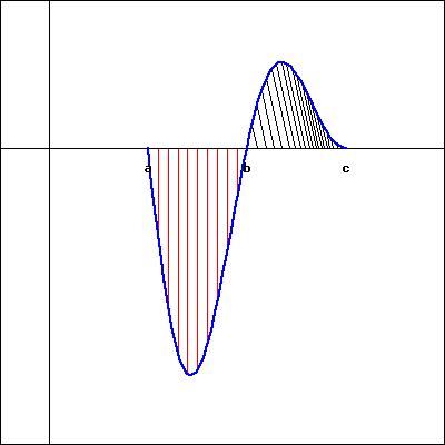 Note that the first area (with vertical, red shading) is 18 and the second (with oblique, black shading) is 6.
- \(\int_a^b f(x) dx = ?\)
- \(\int_b^c f(x) dx = ?\)
- \(\int_a^c f(x) dx = ?\)
- \(\int_a^c |f(x)| dx = ?\)
- Use the graph of \(f(x)\) shown below to find the following integrals.
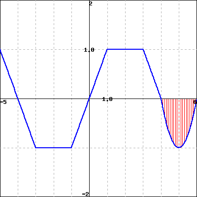
- \(\int_{-4}^0 f(x) dx = ?\)
- If the vertical red shaded area in the graph has area \(A\), estimate \(\int_{-4}^{6} f(x) dx\).
- Suppose \(\displaystyle \int_{-9}^{-4.5} f(x) dx =10, \ \int_{-9}^{-7.5} f(x) dx=8, \ \int_{-6}^{-4.5} f(x)dx =10\).
- \(\displaystyle \int_{-7.5}^{-6} f(x)dx = ?\)
- \(\displaystyle \int_{-6}^{-7.5} (10 f(x)- 8)dx = ?\)
- The velocity of an object moving along an axis is given by the piecewise linear function \(v\) that is pictured in Figure 2.19. Assume that the object is moving to the right when its velocity is positive, and moving to the left when its velocity is negative. Assume that the given velocity function is valid for \(t = 0\) to \(t = 4\).
- Write an expression involving definite integrals whose value is the total change in position of the object on the interval \([0,4]\).
- Use the provided graph of \(v\) to determine the value of the total change in position on \([0,4]\).
- Write an expression involving definite integrals whose value is the total distance traveled by the object on \([0,4]\). What is the exact value of the total distance traveled on \([0,4]\)?
- Find an algebraic formula for the object’s position function on \([0, 1.5]\) that satisfies \(s(0) = 0\).

- Suppose that the velocity of a moving object is given by \(v(t) = t(t-1)(t-3)\), measured in feet per second, and that this function is valid for \(0 \le t \le 4\).
- Write an expression involving definite integrals whose value is the total change in position of the object on the interval \([0,4]\).
- Use appropriate technology to compute Riemann sums to estimate the object’s total change in position on \([0,4]\). Work to ensure that your estimate is accurate to two decimal places, and explain how you know this to be the case.
- Write an expression involving definite integrals whose value is the total distance traveled by the object on \([0,4]\).
- Use appropriate technology to compute Riemann sums to estimate the object’s total distance travelled on \([0,4]\). Work to ensure that your estimate is accurate to two decimal places, and explain how you know this to be the case.
- Consider the graphs of two functions \(f\) and \(g\) that are provided in Figure 2.20. Each piece of \(f\) and \(g\) is either part of a straight line or part of a circle.
- Determine the exact value of \(\int_0^1 [f(x) + g(x)]\,dx\).
- Determine the exact value of \(\int_1^4 [2f(x) - 3g(x)] \, dx\).
- For what constant \(c\) does the following equation hold? \[\begin{equation*} \int_0^4 c \, dx = \int_0^4 [f(x) + g(x)] \, dx \end{equation*}\]

- Let \(f(x) = 3 - x^2\) and \(g(x) = 2x^2\).
- On the interval \([-1,1]\), sketch a labeled graph of \(y = f(x)\) and write a definite integral whose value is the exact area bounded by \(y = f(x)\) on \([-1,1]\).
- On the interval \([-1,1]\), sketch a labeled graph of \(y = g(x)\) and write a definite integral whose value is the exact area bounded by \(y = g(x)\) on \([-1,1]\).
- Write an expression involving a difference of definite integrals whose value is the exact area that lies between \(y = f(x)\) and \(y = g(x)\) on \([-1,1]\).
- Explain why your expression in (c) has the same value as the single integral \(\int_{-1}^1 [f(x) - g(x)] \, dx\).
- Explain why, in general, if \(p(x) \ge q(x)\) for all \(x\) in \([a,b]\), the exact area between \(y = p(x)\) and \(y = q(x)\) is given by \[\begin{equation*} \int_a^b [p(x) - q(x)] \, dx\text{.} \end{equation*}\]
2.4 Summary of main points
- Euler’s method is an algorithm for approximating the solution to an initial value problem by following the tangent lines while we take horizontal steps across the \(t\)-axis.
- If we wish to approximate \(y(\overline{t})\) for some fixed \(\overline{t}\) by taking horizontal steps of size \(\Delta t\), then the error in our approximation is proportional to \(\Delta t\).
- Any Riemann sum of a continuous function \(f\) on an interval \([a,b]\) provides an estimate of the net signed area bounded by the function and the horizontal axis on the interval. Increasing the number of subintervals in the Riemann sum improves the accuracy of this estimate, and letting the number of subintervals increase without bound results in the values of the corresponding Riemann sums approaching the exact value of the enclosed net signed area.
- When we take the limit of Riemann sums, we arrive at what we call the definite integral of \(f\) over the interval \([a,b]\). In particular, the symbol \(\int_a^b f(x) \, dx\) denotes the definite integral of \(f\) over \([a,b]\), and this quantity is defined by the equation \[\begin{equation*} \int_a^b f(x) \, dx = \lim_{n \to \infty} \sum_{i=1}^{n} f(x_i^*) \Delta x\text{,} \end{equation*}\] where \(\Delta x = \frac{b-a}{n}\), \(x_i = a + i\Delta x\) (for \(i = 0, \ldots, n\)), and \(x_i^*\) satisfies \(x_{i-1} \le x_i^* \le x_i\) (for \(i = 1, \ldots, n\)).
- The definite integral \(\int_a^b f(x) \,dx\) measures the exact net signed area bounded by \(f\) and the horizontal axis on \([a,b]\). In the setting where we consider the integral of a velocity function \(v\), \(\int_a^b v(t) \,dt\) measures the exact change in position of the moving object on \([a,b]\); when \(v\) is nonnegative, \(\int_a^b v(t) \,dt\) is the object’s distance traveled on \([a,b]\).
- The definite integral is a sophisticated sum, and thus has some of the same natural properties that finite sums have. Perhaps most important of these is how the definite integral respects sums and constant multiples of functions, which can be summarized by the rule \[\begin{equation*} \int_a^b [c f(x) \pm k g(x)] \,dx = c \int_a^b f(x) \,dx \pm k \int_a^b g(x) \,dx \end{equation*}\] where \(f\) and \(g\) are continuous functions on \([a,b]\) and \(c\) and \(k\) are arbitrary constants.
Euler is pronounced Oy-ler. Among other things, Euler is the mathematician credited with the famous number \(e\).↩︎
What you have seen is essentially an argument which illustrates the Fundamental Theorem of Calculus. We will see it in a more general context in Chapter 3.↩︎
Notice the use of the word “the” rather than “a”. Why do you think this is the case?↩︎
You will likely encounter this in future courses in economics, so getting a sense of what the notation looks like should help in the long term.↩︎
It turns out that a function need not be continuous in order to have a definite integral. For our purposes, we assume that the functions we consider are continuous on the interval(s) of interest. It is straightforward to see that any function that is piecewise continuous on an interval of interest will also have a well-defined definite integral.↩︎